3주차 - 최신 연구 따라잡기 (1)

https://arxiv.org/abs/1907.00235

Autoformer

Auto- Correlation을 활용한 Trandsformer Time-series 의 sesonal와 trend를 분리

추상 요약 (한글 번역)

이 논문은 시계열 데이터의 장기 예측 문제를 연구합니다. 기존의 트랜스포머 기반 모델들은 다양한 self-attention 메커니즘을 사용하여 장기적인 의존성을 파악하려고 합니다. 하지만 복잡한 미래 시계열 패턴은 모델이 정확한 의존성을 찾는 것을 어렵게 만듭니다. 또한, 트랜스포머는 긴 시계열 데이터를 효율적으로 처리하기 위해 point-wise self-attention의 스페어스 버전을 사용해야 하지만, 이는 정보 활용에 있어 병목 현상을 야기합니다. 이러한 문제를 해결하기 위해, 이 논문은 Autoformer라는 새로운 분해 아키텍처와 Auto-Correlation 메커니즘을 제안합니다. 기존의 사전 처리 방식과는 달리, 시계열 분해를 모델 내부의 기본 블록으로 통합하여 복잡한 시계열 데이터에 대한 점진적인 분해 기능을 제공합니다. 또한, 확률 과정 이론에서 영감을 받아 Auto-Correlation 메커니즘을 설계했습니다. 이 메커니즘은 시계열 데이터의 주기에 따라 하위 시계열 단위에서 의존성을 발견하고 표현을 집계합니다. Auto-Correlation은 효율성과 정확성 모두에서 self-attention보다 우수한 성능을 보입니다. 장기 예측에서 Autoformer는 에너지, 교통, 경제, 날씨, 질병 등 다양한 실제 응용 분야를 포함하는 6개의 벤치마크에서 기존 모델에 비해 38% 상대적인 정확도 향상을 달성하며 최첨단 성능을 보여줍니다. 코드는 https://github.com/thuml/Autoformer 에서 확인할 수 있습니다. 핵심 내용:

장기 의존성: 기존 모델은 복잡한 장기적인 패턴을 파악하기 어려움
정보 활용 병목 현상: 스페어스 self-attention은 효율적이지만 정보 활용 제한
Autoformer의 혁신:
- 분해 아키텍처: 기존 사전 처리 방식 혁신, 모델 내부 블록으로 통합
- Auto-Correlation 메커니즘: 하위 시계열 단위에서 의존성 발견 및 표현 집계
결과:
- 다양한 응용 분야에서 최첨단 정확도 달성 (38% 상대적 향상) 요약: 이 논문은 Autoformer라는 새로운 모델을 제안하여 시계열 데이터의 장기 예측 문제를 해결하고 다양한 실제 응용 분야에 적용 가능성을 보여줍니다. 분해 아키텍처와 효율적인 Auto-Correlation 메커니즘은 시계열 데이터 예측 분야에 큰 발전을 가져올 것으로 기대됩니다.

Introduction Time series forecasting has been widely used in energy consumption, traffic and economics planning, weather and disease propagation forecasting. In these real-world applications, one pressing demand is to extend the forecast time into the far future, which is quite meaningful for the long-term planning and early warning. Thus, in this paper, we study the long-term forecasting problem of time series, characterizing itself by the large length of predicted time series. Recent deep forecasting models [41, 17, 20, 28, 23, 29, 19, 35] have achieved great progress, especially the Transformer-based models. Benefiting from the self-attention mechanism, Transformers obtain great advantage in modeling long-term dependencies for sequential data, which enables more powerful big models [7, 11].

도입 (한글 번역)

시계열 데이터 예측은 에너지 소비, 교통 및 경제 계획, 날씨 및 질병 전파 예측 등 다양한 분야에서 널리 사용됩니다. 이러한 실제 응용 분야에서 긴급한 요구 사항 중 하나는 예측 시간을 훨씬 미래까지 확장하는 것입니다. 이는 장기 계획과 조기 경고에 매우 중요합니다. 따라서 이 논문에서는 시간 시리즈의 장기 예측 문제를 연구합니다. 이 문제는 예측된 시간 시리즈의 길이가 긴 특징이 있습니다. 최근의 심층 예측 모델 [41, 17, 20, 28, 23, 29, 19, 35]은 큰 발전을 이루었으며, 특히 트랜스포머 기반 모델들이 눈에 띕니다. 셀프 어텐션 메커니즘으로 인해 트랜스포머는 순차 데이터에 대한 장기 의존성을 모델링하는 데 큰 장점을 가지고 있으며, 이를 통해 더 강력한 대형 모델 [7, 11]을 구축할 수 있습니다. 핵심 내용:

시계열 데이터 예측은 많은 실제 응용 분야에서 중요함
장기 예측은 장기 계획과 조기 경고에 매우 유용함
최근 심층 예측 모델, 특히 트랜스포머 기반 모델들이 발전
트랜스포머는 셀프 어텐션 메커니즘을 통해 장기 의존성 모델링에 강점
이 논문은 트랜스포머 기반 모델을 활용하여 장기 예측 문제 해결

However, the forecasting task is extremely challenging under the long-term setting. First, it is unreliable to discover the temporal dependencies directly from the long-term time series because the dependencies can be obscured by entangled temporal patterns. Second, canonical Transformers with self-attention mechanisms are computationally prohibitive for long-term forecasting because of the quadratic complexity of sequence length. Previous Transformer-based forecasting models [41, 17, 20] mainly focus on improving self-attention to a sparse version. While performance is significantly improved, these models still utilize the point-wise representation aggregation. Thus, in the process of efficiency improvement, they will sacrifice the information utilization because of the sparse point-wise connections, resulting in a bottleneck for long-term forecasting of time series. 복잡한 시간 패턴으로 인한 장기 의존성 파악 어려움:

장기 시계열 데이터에서 직접 시간 의존성을 파악하는 것은 신뢰할 수 없음. 왜냐하면 복잡하게 얽힌 시간 패턴에 의해 의존성이 가려질 수 있기 때문입니다. (이미지: 얽힌 시계열 데이터 그래프)
이러한 복잡한 패턴은 미래의 가치를 예측하는 데 필요한 진정한 의존성을 숨길 수 있습니다. 마치 숲 속의 나무를 한두 개만 보고 숲 전체를 판단하는 것처럼 말이죠. 효율성 vs. 정보 활용 간의 딜레마:
기존 트랜스포머 기반 예측 모델은 주로 스페어스 버전의 self-attention을 개선하는 데 초점을 맞추었습니다. 이를 통해 성능이 크게 향상되었지만, 이러한 모델들은 여전히 포인트별 표현 집계를 사용합니다.
효율성을 높이는 과정에서 스페어스 포인트별 연결로 인해 정보 활용을 희생하게 되어 장기 예측에 한계가 생깁니다. 마치 데이터의 중요한 부분을 무시하고 몇 가지 단점만 보고 전체를 판단하는 것과 같습니다. 핵심 내용:
복잡한 시간 패턴은 장기 예측을 어렵게 만듦
기존 모델들은 효율성과 정보 활용 간의 딜레마에 직면
새로운 모델이 필요함: 장기 의존성을 파악하면서 정보 활용도 높임 이러한 어려움을 극복하기 위해 Autoformer라는 새로운 모델을 제안합니다. Autoformer는 분해 아키텍처와 Auto-Correlation 메커니즘을 사용하여 정보 활용을 유지하면서 효율적으로 장기 의존성을 모델링합니다. 다음 섹션에서 Autoformer의 구조와 작동 방식에 대해 자세히 설명하겠습니다.

To reason about the intricate temporal patterns, we try to take the idea of decomposition, which is a standard method in time series analysis [1, 27]. It can be used to process the complex time series and extract more predictable components. However, under the forecasting context, it can only be used as the pre-processing of past series because the future is unknown [15]. This common usage limits the capabilities of decomposition and overlooks the potential future interactions among decomposed components. Thus, we attempt to go beyond pre-processing usage of decomposition and propose a generic architecture to empower the deep forecasting models with immanent capacity of progressive decomposition. Further, decomposition can ravel out the entangled temporal patterns and highlight the inherent properties of time series [15]. Benefiting from this, we try to take advantage of the series periodicity to renovate the point-wise connection in self-attention. We observe that the sub-series at the same phase position among periods often present similar temporal processes. Thus, we try to construct a series-level connection based on the process similarity derived by series periodicity.

분해와 주기성 활용: 복잡한 시간 패턴 해결

앞 절에서 언급했듯이, 복잡한 시간 패턴은 장기 예측을 어렵게 만듭니다. 이를 해결하기 위해 Autoformer는 두 가지 주요 아이디어를 사용합니다: 1. 분해: 시계열 분석에서 표준적인 방법인 분해를 활용하여 복잡한 시계열 데이터를 더 예측 가능한 구성 요소로 분리합니다. 분해는 데이터의 숨겨진 패턴을 드러내고 예측 모델의 성능을 향상시킬 수 있습니다. (이미지: 시계열 데이터를 분해하여 트렌드, 계절성, 잡음 등으로 구성된 그래프) 그러나 기존의 분해 사용에는 한계가 있습니다:

사전 처리로만 활용: 기존에는 분해를 과거 시계열 데이터의 사전 처리로만 사용했습니다. 왜냐하면 미래는 미지수이기 때문입니다. 이는 분해의 잠재력을 제한합니다.
미래 상호 작용 무시: 기존 사용은 미래의 각 구성 요소 간의 상호 작용을 고려하지 못합니다. Autoformer는 이러한 한계를 극복하기 위해 분해를 혁신적으로 사용합니다:
모델 내부 분해 블록: Autoformer는 분해를 모델 내부의 기본 블록으로 통합합니다. 이를 통해 모델은 시계열 데이터를 점진적으로 분해하면서 미래 시점까지 예측할 수 있습니다. 분해 블록은 마치 프리즘처럼 복잡한 시계열 데이터를 투명하게 만들어 각 구성 요소의 상호 작용을 명확하게 드러냅니다.
주기성 활용: Autoformer는 시계열 데이터의 주기성을 활용하여 유사한 시간 패턴을 가진 하위 시계열 간의 연결을 구축합니다. 마치 시계처럼, 같은 시각의 하위 시계열은 비슷한 변화를 보일 가능성이 높습니다. 이러한 연결은 정보 활용을 유지하면서 장기 예측 효율성을 높입니다. 이를 통해 Autoformer는 복잡한 시간 패턴을 파악하고 미래 시점까지 정확하게 예측할 수 있습니다. 다음 절에서는 Autoformer의 구조와 작동 방식에 대해 더 자세히 설명하겠습니다.

Based on the above motivations, we propose an original Autoformer in place of the Transformers for long-term time series forecasting. Autoformer still follows residual and encoder-decoder structure but renovates Transformer into a decomposition forecasting architecture. By embedding our proposed decomposition blocks as the inner operators, Autoformer can progressively separate the long-term trend information from predicted hidden variables. This design allows our model to alternately decompose and refine the intermediate results during the forecasting procedure. Inspired by the stochastic process theory [8, 24], Autoformer introduces an Auto-Correlation mechanism in place of self-attention, which discovers the sub-series similarity based on the series periodicity and aggregates similar sub-series from underlying periods. This series-wise mechanism achieves $\mathcal{O}(L \log L)$ complexity for length- $L$ series and breaks the information utilization bottleneck by expanding the point-wise representation aggregation to sub-series level. Autoformer achieves the state-of-the-art accuracy on six benchmarks. The contributions are summarized as follows:

To tackle the intricate temporal patterns of the long-term future, we present Autoformer as a decomposition architecture and design the inner decomposition block to empower the deep forecasting model with immanent progressive decomposition capacity.
We propose an Auto-Correlation mechanism with dependencies discovery and information aggregation at the series level. Our mechanism is beyond previous self-attention family and can simultaneously benefit the computation efficiency and information utilization.
Autoformer achieves a 38% relative improvement under the long-term setting on six benchmarks, covering five real-world applications: energy, traffic, economics, weather and disease.

Autoformer: 장기 시계열 예측을 위한 혁신

기존 문제: 복잡한 시간 패턴과 효율성 vs. 정보 활용 간의 딜레마 Autoformer의 핵심 아이디어:

분해 아키텍처: 분해 블록을 모델 내부에 통합하여 점진적으로 시계열 데이터를 분리하고 미래까지 예측
Auto-Correlation 메커니즘: 시계열 주기에 따라 유사한 하위 시계열을 연결하고 정보 활용을 유지하며 효율성 높임 Autoformer의 특징:
트랜스포머 대신 독창적인 아키텍처: 잔여 구조와 인코더-디코더 구조 유지하면서 분해 기능을 통합
점진적 분해: 예측 과정에서 반복적으로 분해를 수행하여 미래 시점까지 정확하게 예측
시계열 주기 활용: 유사한 하위 시계열 간의 연결을 구축하여 정보 활용 확대
효율성과 정보 활용 동시 향상: 시리즈 수준의 정보 집계를 통해 긴 시계열 데이터 처리 효율화
최첨단 정확성: 에너지, 교통, 경제, 날씨, 질병 등 다양한 분야에서 기존 모델보다 38% 향상 Autoformer의 기여:
복잡한 시간 패턴 해결: 분해 아키텍처를 통해 미래까지 정확한 예측
효율적이고 정보 활용이 높은 Auto-Correlation 메커니즘 제안
다양한 실제 응용 분야에서 최첨단 성능 달성 요약: Autoformer는 분해와 주기성을 활용하여 장기 시계열 데이터를 정확하게 예측하는 혁신적인 모델입니다. 이를 통해 에너지, 교통, 경제, 날씨, 질병 등 다양한 분야에서 효과적인 장기 계획과 조기 경고 시스템을 구축할 수 있습니다.

Due to the immense importance of time series forecasting, various models have been well developed. Many time series forecasting methods start from the classic tools [32, 9]. ARIMA [6, 5] tackles the forecasting problem by transforming the non-stationary process to stationary through differencing. The filtering method is also introduced for series forecasting [18, 10]. Besides, recurrent neural networks (RNNs) models are used to model the temporal dependencies for time series [36, 26, 40, 22]. DeepAR [28] combines autoregressive methods and RNNs to model the probabilistic distribution of future series. LSTNet [19] introduces convolutional neural networks (CNNs) with recurrent-skip connections to capture the short-term and long-term temporal patterns. Attention-based RNNs [39, 30, 31] introduce the temporal attention to explore the long-range dependencies for prediction. Also, many works based on temporal convolution networks (TCN) [34, 4, 3, 29] attempt to model the temporal causality with the causal convolution. These deep forecasting models mainly focus on the temporal relation modeling by recurrent connections, temporal attention or causal convolution.

시계열 데이터 예측 모델

시계열 데이터 예측의 중요성으로 인해 다양한 모델들이 개발되었습니다. 많은 예측 모델들은 클래식한 도구들로부터 시작합니다.

ARIMA: 비정상 시계열 데이터를 정상 시계열로 변환하여 예측하는 모델입니다.
필터링 방법: 시계열 데이터를 필터링하여 특정 주기를 강조하고 예측 정확성을 높이는 방법입니다.
순환 신경망 (RNN): 시계열 데이터의 순차적인 특징을 모델링하는 데 효과적인 모델입니다.
DeepAR: 자기회귀 방법과 RNN을 결합하여 미래 시계열 데이터의 확률 분포를 모델링하는 모델입니다.
LSTNet: CNN과 RNN을 결합하여 단기 및 장기 시간 패턴을 모두 포착하는 모델입니다.
어텐션 기반 RNN: 시계열 데이터의 장거리 의존성을 모델링하기 위해 시간적 어텐션 메커니즘을 도입한 모델입니다.
시간 순환 네트워크 (TCN): 시간적인因果관계를 모델링하기 위해 인과적 convolution을 사용하는 모델입니다. 이러한 깊은 예측 모델들은 주로 순환 연결, 시간적 어텐션, 인과적 convolution 등을 통해 시간 관계를 모델링합니다.

attention and also achieves $\mathcal{O}(L \log L)$ complexity. Note that these methods are based on the vanilla Transformer and try to improve the self-attention mechanism to a sparse version, which still follows the point-wise dependency and aggregation. In this paper, our proposed Auto-Correlation mechanism is based on the inherent periodicity of time series and can provide series-wise connections.

트랜스포머와 장기 시계열 예측

최근 트랜스포머 모델은 자연어 처리, 음성 처리, 이미지 인식 등 다양한 분야에서 뛰어난 성능을 보여주었습니다.
하지만 자기-어텐션 메커니즘을 사용하는 트랜스포머를 장기 시계열 예측에 적용하는 것은 계산 비용이 높은 문제가 있습니다. 시계열 데이터의 길이가 길어질수록 메모리와 시간 복잡성이 제곱급으로 증가하기 때문입니다.
LogTrans, Reformer, Informer 등 기존 연구들은 스페어스 자기-어텐션 기반으로 계산 효율을 높이려고 노력했습니다. 이 방법들은 시계열 데이터의 일부 부분만 고려하여 복잡성을 O(L(logL)2) 또는 O(LlogL)로 줄이지만, 여전히 데이터 간의 점별적인 의존성과 집계 방식을 유지합니다.
Autoformer는 이러한 한계를 극복하기 위해 시계열 데이터의 주기성을 활용한 Auto-Correlation 메커니즘을 제안합니다. 이 메커니즘은 시계열 데이터의 유사한 하위 시계열 간의 연결을 구축하여 정보 활용을 유지하면서 효율성을 높입니다. 핵심 내용:
기존 연구들은 스페어스 자기-어텐션을 통해 효율성을 높이려고 노력했으나 정보 활용이 제한됨
Autoformer는 시계열 주기를 활용한 Auto-Correlation 메커니즘을 제안하여 시리즈 수준의 연결을 구축하고 정보 활용 유지
이를 통해 Autoformer는 장기 시계열 예측에 효과적이며 계산 효율성도 높임

Decomposition of Time Series As a standard method in time series analysis, time series decomposition [1, 27] deconstructs a time series into several components, each representing one of the underlying categories of patterns that are more predictable. It is primarily useful for exploring historical changes over time. For the forecasting tasks, decomposition is always used as the pre-processing of historical series before predicting future series [15, 2], such as Prophet [33] with trend-seasonality decomposition and N-BEATS [23] with basis expansion and DeepGLO [29] with matrix decomposition. However, such pre-processing is limited by the plain decomposition effect of historical series and overlooks the hierarchical interaction between the underlying patterns of series in the long-term future. This paper takes the decomposition idea from a new progressive dimension. Our Autoformer harnesses the decomposition as an inner block of deep models, which can progressively decompose the hidden series throughout the whole forecasting process, including both the past series and the predicted intermediate results.

시계열 데이터 분해

시계열 데이터 분해 [1, 27]는 복잡한 시계열 데이터를 예측 가능한 성분들로 분리하는 표준적인 방법입니다. 이는 추세, 계절성, 잡음 등과 같은 기본적인 패턴을 이해하고 예측하는 데 유용합니다.
과거 시계열 데이터 분석에 주로 사용되었던 기존 분해 방법은 다음과 같은 한계점이 있습니다.
사전 처리로만 활용: 기존에는 분해를 예측 전에 과거 시계열 데이터의 사전 처리로만 사용했습니다.
미래 상호 작용 무시: 단순한 분해로 인해 미래 시점에서 각 구성 요소 간의 상호 작용을 고려하지 못했습니다. Autoformer는 이러한 한계를 극복하기 위해 분해를 혁신적으로 사용
모델 내부 분해 블록: Autoformer는 분해 기능을 모델 내부의 블록으로 통합합니다. 이를 통해 모델은 과거 시계열 데이터뿐만 아니라 예측된 중간 결과까지 점진적으로 분해할 수 있습니다. 마치 시계를 멈추고 각 부품을 검사하면서 미래 시계의 작동을 예측하는 것과 같습니다.
점진적 분해: Autoformer는 예측 과정에서 반복적으로 분해를 수행하여 미래 시점까지 정확하게 예측할 수 있습니다. 이는 단순한 사전 처리 분해보다 미래 시점에서 각 구성 요소 간의 상호 작용을 고려할 수 있습니다. 핵심 내용:
기존 분해 방법은 사전 처리로만 활용되어 한계가 있었음
Autoformer는 분해 기능을 모델 내부 블록으로 통합하여 시계열 데이터를 점진적으로 분해하고 미래 상호 작용을 고려함
이를 통해 Autoformer는 더 정확한 장기 예측을 수행할 수 있음

\section{Autoformer} The time series forecasting problem is to predict the most probable length- $O$ series in the future given the past length- $I$ series, denoting as input-I-predict-O $O$ . The long-term forecasting setting is to predict the long-term future, i.e. larger $O$ . As aforementioned, we have highlighted the difficulties of long-term series forecasting: handling intricate temporal patterns and breaking the bottleneck of computation efficiency and information utilization. To tackle these two challenges, we introduce the decomposition as a builtin block to the deep forecasting model and propose Autoformer as a decomposition architecture. Besides, we design the Auto-Correlation mechanism to discover the period-based dependencies and aggregate similar sub-series from underlying periods.

Autoformer: 장기 시계열 데이터 예측 모델

Autoformer는 과거 시계열 데이터(길이 I)를 바탕으로 미래 시계열 데이터(길이 O)를 예측하는 모델입니다. 특히, 장기 예측은 미래 시점이 더 멀리, 즉 O가 더 큰 경우를 말합니다. 앞서 언급했듯이, 장기 예측은 두 가지 어려움에 직면합니다: 복잡한 시간 패턴 처리와 계산 효율 vs. 정보 활용 간의 딜레마. 이러한 문제를 해결하기 위해, Autoformer는 다음과 같은 핵심 아이디어를 사용합니다:

분해 내장 아키텍처: 분해 기능을 모델 내부 블록으로 통합하여 과거 시계열 데이터와 예측된 중간 결과를 모두 점진적으로 분해합니다.
Auto-Correlation 메커니즘: 시계열 데이터의 주기에 따라 유사한 하위 시계열 간의 연결을 구축하여 정보 활용을 유지하면서 계산 효율을 높입니다. Autoformer의 특징:
잔여 구조와 인코더-디코더 구조 유지: 기존 트랜스포머와 유사한 구조를 유지하면서 분해 기능을 통합
점진적 분해: 예측 과정에서 반복적으로 분해를 수행하여 미래 시점까지 정확하게 예측
효율적인 Auto-Correlation 메커니즘: 시계열 주기를 활용하여 유사한 하위 시계열 간의 연결을 구축, 계산 비용 절감
시리즈 수준의 정보 집계: 하위 시계열 간의 유사성을 고려하여 정보 활용 확대 요약: Autoformer는 분해 아키텍처와 효율적인 Auto-Correlation 메커니즘을 활용하여 복잡한 시간 패턴을 해결하고 정확한 장기 예측을 수행하는 모델입니다. 이는 에너지, 교통, 경제, 날씨, 질병 등 다양한 실제 응용 분야에서 효과적으로 활용될 수 있습니다.

Autoformer는 기존 트랜스포머 아키텍처를 개선하여 분해 기능을 통합한 “깊은 분해 아키텍처”를 제안합니다. 이 아키텍처는 다음 세 가지 주요 구성 요소로 이루어집니다:

내부 시계열 분해 블록: 이 블록은 시계열 데이터를 점진적으로 분해하여 미래 시점까지 정확한 예측을 가능하게 합니다. 마치 렌즈를 통해 복잡한 시계열 데이터를 투명하게 만들어 각 구성 요소를 명확하게 드러내는 역할을 합니다.
Auto-Correlation 메커니즘: 이 메커니즘은 시계열 데이터의 주기에 따라 유사한 하위 시계열 간의 연결을 구축합니다. 이를 통해 정보 활용을 유지하면서 계산 비용을 절감할 수 있습니다. 마치 시계의 바늘이 같은 시간대에 비슷한 위치를 가질 가능성이 높은 것처럼, Auto-Correlation은 유사한 하위 시계열 간의 의존성을 효율적으로 모델링합니다.
인코더 및 디코더: 이들은 기존 트랜스포머에서 사용하는 익숙한 구조입니다. 인코더는 과거 시계열 데이터를 처리하고, 디코더는 예측된 결과를 생성합니다.

Series decomposition block To learn with the complex temporal patterns in long-term forecasting context, we take the idea of decomposition [1, 27], which can separate the series into trend-cyclical and seasonal parts. These two parts reflect the long-term progression and the seasonality of the series respectively. However, directly decomposing is unrealizable for future series because the future is just unknown. To tackle this dilemma, we present a series decomposition block as an inner operation of Autoformer (Figure 17), which can extract the long-term stationary trend from predicted intermediate hidden variables progressively. Concretely, we adapt the moving average to smooth out periodic fluctuations and highlight the long-term trends. For length- $L$ input series $\mathcal{X} \in \mathbb{R}^{L \times d}$ , the process is:

\begin{aligned} & \mathcal{X}{\mathrm{t}}=\operatorname{AvgPool}(\operatorname{Padding}(\mathcal{X})) \\ & \mathcal{X}{\mathrm{s}}=\mathcal{X}-\mathcal{X}_{\mathrm{t}} \end{aligned}

where $\mathcal{X}{\mathrm{s}}, \mathcal{X}{\mathrm{t}} \in \mathbb{R}^{L \times d}$ denote the seasonal and the extracted trend-cyclical part respectively. We adopt the $\operatorname{Avg} \operatorname{Pool}(\cdot)$ for moving average with the padding operation to keep the series length unchanged. We use $\mathcal{X}{\mathrm{s}}, \mathcal{X}{\mathrm{t}}=\operatorname{SeriesDecomp}(\mathcal{X})$ to summarize above equations, which is a model inner block. 장기 시계열 예측에서 복잡한 시간 패턴을 다루기 위해 Autoformer는 시계열 데이터를 추세-주기적 성분과 계절성 성분으로 분해하는 분해 개념을 도입합니다. 추세-주기적 성분은 시계열 데이터의 장기적인 변화를 나타내고, 계절성 성분은 일정한 주기에 반복되는 패턴을 나타냅니다. 하지만 미래는 알 수 없기 때문에 미래 시계열 데이터를 직접 분해하는 것은 불가능합니다. 이러한 딜레마를 해결하기 위해 Autoformer는 모델 내부 작동 방식인 시계열 분해 블록을 제안합니다 (그림 17 참조). 이 블록은 예측된 중간 숨겨진 변수에서 점진적으로 장기적인 정상적인 추세를 추출합니다. 구체적으로, Autoformer는 이동 평균 필터를 사용하여 주기적인 변동을 부드럽게 만들고 장기적인 추세를 명확하게 드러냅니다. 길이가 L인 입력 시계열 데이터 X∈RL×d에 대해 다음과 같은 과정을 수행합니다:

\begin{aligned} & \mathcal{X}{\mathrm{t}}=\operatorname{AvgPool}(\operatorname{Padding}(\mathcal{X})) \ & \mathcal{X}{\mathrm{s}}=\mathcal{X}-\mathcal{X}_{\mathrm{t}} \end{aligned}

여기에서 Xs,Xt∈RL×d는 각각 계절성 부분과 추출된 추세-주기적 부분을 나타냅니다. AvgPool(⋅)은 이동 평균 필터에 패딩 작업을 추가하여 시계열 데이터의 길이를 유지합니다. 이러한 방식을 Xs,Xt=SeriesDecomp(X)로 요약하여 모델 내부 블록으로 사용합니다. 핵심 내용:

시계열 분해 블록은 시계열 데이터를 추세-주기적 성분과 계절성 성분으로 분해합니다.
이 블록은 예측된 중간 결과에서 점진적으로 장기적인 추세를 추출합니다.
이동 평균 필터를 사용하여 시계열 데이터의 주기적인 변동을 부드럽게 만듭니다.

요약

시계열 분해 블록은 Autoformer의 핵심 구성 요소 중 하나이며, 복잡한 시간 패턴을 효과적으로 다루고 정확한 장기 예측을 수행하는 데 중요한 역할을 합니다.

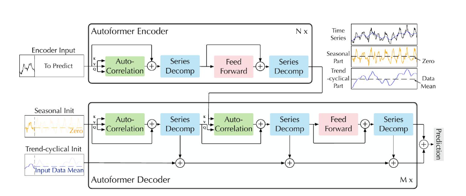
Autoformer 모델 입력

Autoformer는 과거 시계열 데이터를 활용하여 미래 시점을 예측하는 모델입니다. 모델은 두 부분으로 나눌 수 있습니다: 인코더와 디코더. 인코더 입력:

과거 I 개의 시계열 데이터 Xen ∈RI×d를 입력으로 받습니다. 디코더 입력:
분해 아키텍처 특징으로 인해, 디코더는 두 가지 부분의 입력을 받습니다:
- 계절성 성분 Xdes ∈R(2I+O)×d: 과거 정보를 최대한 유지하기 위해, 인코더 입력의 후반부를 분해하여 얻은 길이 2I 의 데이터를 사용하고, 나머지 길이 O만큼은 0으로 채운 플레이스홀더를 사용합니다.
- 추세-주기적 성분 Xdet ∈R(2I+O)×d: 인코더 입력을 분해하여 얻은 추세-주기적 성분 데이터를 사용하고, 나머지 길이 O만큼은 시계열 데이터의 평균값으로 채운 플레이스홀더를 사용합니다. 요약:
인코더는 과거 시계열 데이터 전체를 입력으로 받습니다.
디코더는 과거 시계열 데이터의 일부 분해된 정보와 플레이스홀더를 입력으로 받습니다. 이를 통해 미래 시점을 예측하기 위한 정보를 효율적으로 활용합니다.

핵심 내용

Autoformer는 분해 아키텍처를 사용하여 시계열 데이터의 과거 정보를 최대한 유지하면서 미래 시점을 예측합니다. 이는 계절성 성분과 추세-주기적 성분을 별도로 처리하고, 미래 시점에 대한 정보 부족을 플레이스홀더를 통해 해결합니다.

Encoder As shown in Figure 1, the encoder focuses on the seasonal part modeling. The output of the encoder contains the past seasonal information and will be used as the cross information to help the decoder refine prediction results. Suppose we have $N$ encoder layers. The overall equations for $l$ -th encoder layer are summarized as $\mathcal{X}*{\text {en }}^{l}=\operatorname{Encoder}\left(\mathcal{X}*{\text {en }}^{l-1}\right)$ . Details are shown as follows:

\begin{aligned} & \mathcal{S}{\mathrm{en}}^{l, 1},{ }{-}=\operatorname{SeriesDecomp}\left(\text { Auto-Correlation }\left(\mathcal{X}{\mathrm{en}}^{l-1}\right)+\mathcal{X}{\mathrm{en}}^{l-1}\right) \\ & \mathcal{S}{\mathrm{en}}^{l, 2},{ }{-}=\operatorname{SeriesDecomp}\left(\operatorname{FeedForward}\left(\mathcal{S}{\mathrm{en}}^{l, 1}\right)+\mathcal{S}{\mathrm{en}}^{l, 1}\right) \end{aligned}

where ” ” is the eliminated trend part. $\mathcal{X}*{\text {en }}^{l}=\mathcal{S}*{\text {en }}^{l, 2}, l \in\{1, \cdots, N\}$ denotes the output of $l$ -th encoder layer and $\mathcal{X}*{\text {en }}^{0}$ is the embedded $\mathcal{X}*{\text {en }} . \mathcal{S}_{\text {en }}^{l, i}, i \in\{1,2\}$ represents the seasonal component after the $i$ -th series decomposition block in the $l$ -th layer respectively. We will give detailed description of Auto-Correlation $(\cdot)$ in the next section, which can seamlessly replace the self-attention.

Autoformer의 인코더

Autoformer는 시계열 데이터의 계절적인 특징을 효과적으로 모델링하기 위해 인코더 부분을 사용합니다. 인코더는 과거 시계열 데이터의 계절성 정보를 추출하고, 이 정보는 디코더에서 예측 결과를 개선하는 데 사용됩니다. 인코더는 N 개의 레이어로 구성됩니다. 각 레이어는 다음과 같은 과정을 수행합니다:

시계열 분해 및 Auto-Correlation:

먼저, 이전 레이어의 출력 Xen l−1에 Auto-Correlation을 적용하여 유사한 하위 시계열 간의 연결을 구축합니다.
이후 SeriesDecomp 블록을 사용하여 연결된 데이터와 이전 레이어의 출력을 분해하여 계절성 성분 (Senl,1)과 추세-주기적 성분을 분리합니다. 추세-주기적 성분은 이 과정에서 버려집니다.

FeedForward 네트워크:

추출된 계절성 성분 Senl,1을 FeedForward 네트워크에 통과시켜 정보 추출 및 변환을 수행합니다.
이후 SeriesDecomp 블록을 다시 사용하여 변환된 계절성 성분을 분해하여 최종 계절성 정보 Senl,2를 얻습니다. 이러한 과정을 반복하여 인코더는 과거 시계열 데이터의 계절성 특징을 점진적으로 추출하고 정제합니다. 이 추출된 정보는 디코더에서 미래 시점을 예측하는 데 중요한 역할을 합니다. 핵심 내용:
인코더는 시계열 데이터의 계절성 특징을 효과적으로 모델링합니다.
Auto-Correlation 메커니즘을 사용하여 유사한 하위 시계열 간의 연결을 구축합니다.
SeriesDecomp 블록을 사용하여 계절성 성분과 추세-주기적 성분을 분리합니다.
추출된 계절성 정보는 디코더에서 미래 시점 예측에 활용됩니다. 주의사항:
Auto-Correlation에 대한 자세한 설명은 다음 섹션에서 다룰 예정입니다.
” “은 시계열 분해 블록에서 제거된 추세-주기적 성분을 나타냅니다.

요약

Autoformer의 인코더는 시계열 데이터의 계절성 특징을 효과적으로 추출하고 정제하여 디코더에서 미래 시점 예측에 활용합니다. 이는 정확한 장기 시계열 예측을 가능하게 하는 핵심 요소 중 하나입니다.

Decoder The decoder contains two parts: the accumulation structure for trend-cyclical components and the stacked Auto-Correlation mechanism for seasonal components (Figure 11). Each decoder layer contains the inner Auto-Correlation and encoder-decoder Auto-Correlation, which can refine the prediction and utilize the past seasonal information respectively. Note that the model extracts the potential trend from the intermediate hidden variables during the decoder, allowing Autoformer to progressively refine the trend prediction and eliminate interference information for period-based dependencies discovery in Auto-Correlation. Suppose there are $M$ decoder layers. With the latent variable $\mathcal{X}*{\mathrm{en}}^{N}$ from the encoder, the equations of $l$ -th decoder layer can be summarized as $\mathcal{X}*{\mathrm{de}}^{l}=$ $\operatorname{Decoder}\left(\mathcal{X}*{\mathrm{de}}^{l-1}, \mathcal{X}*{\mathrm{en}}^{N}\right)$ . The decoder can be formalized as follows:

\begin{aligned} \mathcal{S}*{\mathrm{de}}^{l, 1}, \mathcal{T}*{\mathrm{de}}^{l, 1} & =$\operatorname{SeriesDecomp}\left(\text { Auto-Correlation }\left(\mathcal{X}{\mathrm{de}}^{l-1}\right)+\mathcal{X}{\mathrm{de}}^{l-1}\right) \\ \mathcal{S}{\mathrm{de}}^{l, 2}, \mathcal{T}{\mathrm{de}}^{l, 2} $& $=\operatorname{SeriesDecomp}\left(\text { Auto-Correlation }\left(\mathcal{S}{\mathrm{de}}^{l, 1}, \mathcal{X}{\mathrm{en}}^{N}\right)+\mathcal{S}{\mathrm{de}}^{l, 1}\right) \\ \mathcal{S}{\mathrm{de}}^{l, 3}, \mathcal{T}{\mathrm{de}}^{l, 3} $*& =\operatorname{SeriesDecomp}\left(\text { FeedForward }\left(\mathcal{S}*{\mathrm{de}}^{l, 2}\right)+\mathcal{S}*{\mathrm{de}}^{l, 2}\right) \\ \mathcal{T}*{\mathrm{de}}^{l} & =\mathcal{T}*{\mathrm{de}}^{l-1}+\mathcal{W}*{l, 1} * \mathcal{T}*{\mathrm{de}}^{l, 1}+\mathcal{W}*{l, 2} * \mathcal{T}*{\mathrm{de}}^{l, 2}+\mathcal{W}*{l, 3} * \mathcal{T}_{\mathrm{de}}^{l, 3} \end{aligned}

where $\mathcal{X}{\mathrm{de}}^{l}=\mathcal{S}{\mathrm{de}}^{l, 3}, l \in\{1, \cdots, M\}$ denotes the output of $l$ -th decoder layer. $\mathcal{X}*{\mathrm{de}}^{0}$ is embedded from $\mathcal{X}*{\text {des }}$ for deep transform and $\mathcal{T}*{\mathrm{de}}^{0}=\mathcal{X}*{\text {det }}$ is for accumulation. $\mathcal{S}*{\mathrm{de}}^{l, i}, \mathcal{T}*{\mathrm{de}}^{l, i}, i \in\{1,2,3\}$ represent the seasonal component and trend-cyclical component after the $i$ -th series decomposition block in the $l$ -th layer respectively. $\mathcal{W}*{l, i}, i \in\{1,2,3\}$ represents the projector for the $i$ -th extracted trend $\mathcal{T}*{\text {de }}^{l, i}$ .

ㄴ 이 텍스트는 시계열 데이터 분석을 위한 복잡한 디코더 메커니즘에 대해 설명하고 있습니다. 이 디코더는 트렌드-주기적 요소와 계절적 요소를 분석하기 위해 두 부분으로 구성되어 있습니다.
1. 트렌드-주기적 요소를 위한 축적 구조(Accumulation Structure): 이 부분은 데이터의 트렌드(장기적 경향)와 주기적 변화를 분석합니다.
2. 계절적 요소를 위한 스택드 자기상관 메커니즘(Stacked Auto-Correlation Mechanism): 이는 정기적으로 반복되는 계절적 패턴을 처리하기 위해 사용 각 디코더 레이어 - 예측을 정제하고 과거 계절 정보를 활용
- 내부 자기상관(Inner Auto-Correlation)
- 인코더-디코더 자기상관(Encoder-Decoder Auto-Correlation)을 이를 통해 할 수 있습니다. 디코더는 중간 숨겨진 변수에서 잠재적인 트렌드를 추출하여 Autoformer가 트렌드 예측을 점진적으로 정제하고 주기적 의존성 발견을 위한 방해 정보를 제거할 수 있게 합니다. 디코더 레이어는 다음과 같이 정식화됩니다:

\mathcal{S}{\mathrm{de}}^{l, 1}, \mathcal{T}{\mathrm{de}}^{l, 1}, \ldots

여기서 각각의 시리즈 분해 블록 후에 계절적 요소( $\mathcal{S}*{\mathrm{de}}^{l, i}$ )와 트렌드-주기적 요소( $\mathcal{T}*{\mathrm{de}}^{l, i}$ )를 나타냅니다. 각 레이어의 출력은 $\mathcal{X}{\mathrm{de}}^{l}=\mathcal{S}{\mathrm{de}}^{l, 3}$ 로 표현됩니다. 여기서 $l$ 은 1부터 $M$ 까지의 디코더 레이어를 나타냅니다. 디코더는 각 레이어에서 트렌드와 계절적 요소를 분해하고 재조합하여 시계열 데이터의 특성을 더 정확하게 예측하고 분석하는 데 사용됩니다.

Autoformer의 디코더

Autoformer의 디코더는 두 가지 부분으로 구성됩니다: 1. 추세-주기적 성분 누적 구조:

추세-주기적 성분은 미래 시점에 대한 장기적인 변화를 나타냅니다.
디코더는 이러한 성분을 누적하여 점차적으로 미래 시점의 추세를 예측합니다.
각 레이어는 이전 레이어의 추세-주기적 성분을 받아들이고 새로운 정보를 추가하여 더 정확한 예측을 생성합니다. 2. 스택된 Auto-Correlation 메커니즘:
계절성 성분은 일정한 주기에 반복되는 패턴을 나타냅니다.
디코더는 스택된 Auto-Correlation 메커니즘을 사용하여 과거 시계열 데이터의 계절성 정보와 유사한 하위 시계열 간의 연결을 구축합니다.
이를 통해 미래 시점의 계절성 패턴을 예측하고 더 정확한 예측 결과를 생성합니다. 디코더 레이어의 주요 기능:
시계열 분해: 각 레이어는 이전 레이어의 출력을 SeriesDecomp 블록을 사용하여 계절성 성분과 추세-주기적 성분으로 분리합니다.
Auto-Correlation: Auto-Correlation 메커니즘을 사용하여 유사한 하위 시계열 간의 연결을 구축하여 정보 활용을 유지하면서 계산 비용을 절감합니다.
FeedForward 네트워크: 추출된 계절성 성분을 FeedForward 네트워크에 통과시켜 정보 추출 및 변환을 수행합니다.
누적 구조: 추세-주기적 성분을 누적하여 미래 시점의 추세를 점진적으로 예측합니다.
인코더 정보 활용: 인코더에서 추출된 계절성 정보를 사용하여 디코더의 예측 정확도를 높입니다. 디코더의 핵심 이점:
장기적인 추세 변화를 효과적으로 모델링합니다.
계절성 패턴을 정확하게 예측합니다.
Auto-Correlation 메커니즘을 사용하여 정보 활용을 유지하면서 계산 비용을 절감합니다. 주의사항:
” “은 시계열 분해 블록에서 제거된 추세-주기적 성분을 나타냅니다.
Wl,i,i∈{1,2,3}은 각 추출된 추세 성분을 투영하는 프로젝터입니다. 요약: Autoformer의 디코더는 추세-주기적 성분 누적 구조와 스택된 Auto-Correlation 메커니즘을 사용하여 장기적인 시계열 데이터를 정확하게 예측합니다. 이는 에너지, 교통, 경제, 날씨, 질병 등 다양한 분야에서 효과적으로 활용될 수 있습니다.

\subsection{Auto-Correlation Mechanism} As shown in Figure 2, we propose the Auto-Correlation mechanism with series-wise connections to expand the information utilization. Auto-Correlation discovers the period-based dependencies by calculating the series autocorrelation and aggregates similar sub-series by time delay aggregation.

Auto-Correlation 메커니즘: 시계열 정보 활용 확대

Autoformer는 시계열 데이터의 복잡한 패턴을 해결하기 위해 Auto-Correlation 메커니즘을 제안합니다. 이 메커니즘은 기존 트랜스포머의 자기-어텐션 메커니즘과 달리, 시계열 데이터의 고유한 특징을 고려하여 다음과 같은 두 가지 기능을 수행합니다:

주기-기반 의존성 발견: 시계열 데이터는 종종 특정 주기에 반복되는 패턴을 가지고 있습니다. Auto-Correlation은 이러한 주기-기반 의존성을 계산하여 서로 유사한 하위 시계열 간의 연결을 구축합니다. 이를 통해 과거 시계열 데이터의 정보를 효과적으로 활용하여 더 정확한 예측을 수행할 수 있습니다.
유사한 하위 시계열 집계: Auto-Correlation은 시간 지연 집계를 통해 유사한 하위 시계열을 하나로 통합합니다. 이를 통해 계산 비용을 절감하면서도 정보 활용을 유지할 수 있습니다. Auto-Correlation 메커니즘은 다음과 같은 세 가지 단계로 구성됩니다:
시계열 자기-상관 계산: 시계열 데이터의 각 시점에 대해 자기-상관 계수를 계산하여 서로 유사한 하위 시계열을 식별합니다.
시간 지연 집계: 계산된 자기-상관 계수를 기준으로 유사한 시점들을 그룹화하여 하나의 대표 시계열로 집계합니다.
정보 활용: 집계된 시계열을 다음 단계의 계산에 활용하여 시계열 예측을 수행합니다. Auto-Correlation 메커니즘의 장점:

시계열 데이터의 주기-기반 의존성을 고려하여 정보 활용을 확대합니다.
계산 비용을 절감하면서 정확한 예측을 수행할 수 있습니다.
기존 트랜스포머의 자기-어텐션 메커니즘보다 시계열 데이터의 특징을 효과적으로 반영합니다. Auto-Correlation 메커니즘은 Autoformer의 핵심 요소 중 하나이며, 시계열 데이터의 복잡한 패턴을 효과적으로 모델링하여 정확한 장기 예측을 수행하는 데 중요한 역할을 합니다. 주의사항:
본 설명은 Auto-Correlation 메커니즘의 개요를 제공합니다. 더 자세한 내용은 논문을 참조하시기 바랍니다. 요약: Auto-Correlation 메커니즘은 시계열 데이터의 주기-기반 의존성을 고려하여 정보 활용을 확대하고 계산 비용을 절감합니다. 이는 Autoformer의 정확한 장기 예측 성능에 중요한 역할을 합니다.

Period-based dependencies It is observed that the same phase position among periods naturally provides similar sub-processes. Inspired by the stochastic process theory [8, 24], for a real discretetime process $\left\{\mathcal{X}*{t}\right\}$ , we can obtain the autocorrelation $\mathcal{R}*{\mathcal{X X}}(\tau)$ by the following equations:

\mathcal{R}*{\mathcal{X X}}(\tau)=\lim {L \rightarrow \infty} \frac{1}{L} \sum{t=1}^{L} \mathcal{X}*{t} \mathcal{X}_{t-\tau}

$\mathcal{R}*{\mathcal{X X}}(\tau)$ reflects the time-delay similarity between $\left\{\mathcal{X}*{t}\right\}$ and its $\tau$ lag series $\left\{\mathcal{X}*{t-\tau}\right\}$ . As shown in Figure 2, we use the autocorrelation $\mathcal{R}(\tau)$ as the unnormalized confidence of estimated period length $\tau$ . Then, we choose the most possible $k$ period lengths $\tau*{1}, \cdots, \tau_{k}$ . The period-based dependencies are derived by the above estimated periods and can be weighted by the corresponding autocorrelation.

이 문단은 시간에 따른 데이터의 반복 패턴을 분석하는 방법에 대해 설명하고 있습니다. 이 내용은 시계열 데이터 분석에서 중요한 개념인 ‘자기상관’에 관한 것입니다. 자기상관은 시간에 따라 변화하는 데이터 집합(예: 주식 가격, 기온 등)에서, 시간 지연(τ)에 따라 데이터가 얼마나 유사한지를 측정합니다. 여기서 사용된 주요 방정식은 자기상관을 계산하는 공식입니다:

$\mathcal{R}{\mathcal{X X}}(\tau)=\lim {L \rightarrow \infty} \frac{1}{L} \sum{t=1}^{L} \mathcal{X}{t} \mathcal{X}_{t-\tau}$

이 공식은 시간 지연 τ에 대해 데이터 집합 $\left\{\mathcal{X}*{t}\right\}$ 의 현재 값과 τ 시간만큼 지연된 값 사이의 유사성을 측정합니다. 이 방법을 사용하여, 데이터에서 반복되는 패턴의 주기(τ)를 추정할 수 있습니다. 추정된 여러 주기(τ1, τ2, …, τk) 중에서 가장 가능성이 높은 k개의 주기를 선택합니다. 이렇게 추정된 주기들은 해당 주기들의 자기상관에 의해 가중치를 받으며, 이를 통해 데이터의 주기적 의존성을 분석할 수 있습니다. 간단히 말해, 이 방법은 시간에 따른 데이터에서 주기적으로 반복되는 패턴을 찾아내고, 이러한 패턴의 강도와 중요성을 평가하는 데 사용됩니다.

주기 기반 의존성: 시간 지연을 이용한 정보 활용

자동 예측 모델인 Autoformer는 시계열 데이터의 주기적인 패턴을 효과적으로 포착하기 위해 주기-기반 의존성이라는 개념을 사용합니다. 이 개념은 다음과 같은 핵심 내용을 포함합니다: 1. 유사한 시점 간의 연관성: 시계열 데이터에서 같은 주기에 해당하는 시점들은 종종 유사한 특징을 가지고 있습니다. 예를 들어, 일년 주기의 데이터에서 봄과 봄은 비슷한 패턴을 보여줄 가능성이 높습니다. 2. 시간 지연 상호관계: Autoformer는 이러한 유사성을 측정하기 위해 자기-상관 계수를 사용합니다. 자기-상관 계수는 시계열 데이터와 그 자신을 일정 시간 지연시킨 시계열 데이터 사이의 상관 관계를 나타냅니다. 높은 자기-상관 계수는 두 시점 간의 유사성이 강하다는 것을 의미합니다. 3. 주기 추정: Autoformer는 계산된 자기-상관 계수를 기반으로 시계열 데이터의 주기를 추정합니다. 주기는 데이터에서 반복되는 패턴의 길이를 말하며, 높은 자기-상관 계수를 나타내는 시간 지연이 주기의 길이가 될 가능성이 높습니다. 4. 유사한 하위 시계열 그룹화: 추정된 주기에 따라 Autoformer는 유사한 시점들을 그룹으로 묶어 하나의 하위 시계열로 만듭니다. 이를 통해 모델은 각 주기 내의 패턴을 더 효과적으로 학습할 수 있습니다. 5. 가중치 적용: Autoformer는 자기-상관 계수를 사용하여 각 주기의 중요성을 나타내는 가중치를 적용합니다. 더 높은 자기-상관 계수를 가진 주기는 더 큰 가중치를 받아 예측 과정에서 더 중요한 정보로 활용됩니다. 핵심 이점:

주기-기반 의존성을 활용하여 시계열 데이터의 복잡한 패턴을 효과적으로 모델링합니다.
유사한 시점 간의 정보를 효율적으로 활용하여 더 정확한 예측을 수행합니다.
시간 지연을 사용하여 계산 비용을 절감하면서 정보 활용을 유지합니다. 요약: Autoformer의 주기-기반 의존성은 시계열 데이터의 주기적인 특징을 효과적으로 활용하여 장기적인 시계열 예측 성능을 향상시키는 중요한 기술입니다. 이를 통해 에너지, 교통, 경제, 날씨 등 다양한 분야에서 더 정확한 예측을 수행할 수 있습니다. 주의사항:
본 설명은 주기-기반 의존성의 개요를 제공합니다. 더 자세한 내용은 논문을 참조하시기 바랍니다.

Time delay aggregation The period-based dependencies connect the sub-series among estimated periods. Thus, we present the time delay aggregation block (Figure 2), which can roll the series based on selected time delay $\tau_{1}, \cdots, \tau_{k}$ . This operation can align similar sub-series that are at the same phase position of estimated periods, which is different from the point-wise dot-product aggregation in self-attention family. Finally, we aggregate the sub-series by softmax normalized confidences. For the single head situation and time series $\mathcal{X}$ with length- $L$ , after the projector, we get query $\mathcal{Q}$ , key $\mathcal{K}$ and value $\mathcal{V}$ . Thus, it can replace self-attention seamlessly. The Auto-Correlation mechanism is:

\begin{aligned} \tau_{1}, \cdots, \tau_{k} & =\underset{\tau \in\{1, \cdots, L\}}{\arg \operatorname{Topk}}\left(\mathcal{R}*{\mathcal{Q}, \mathcal{K}}(\tau)\right) \\ \widehat{\mathcal{R}}*{\mathcal{Q}, \mathcal{K}}\left(\tau_{1}\right), \cdots, \widehat{\mathcal{R}}*{\mathcal{Q}, \mathcal{K}}\left(\tau*{k}\right) & =\operatorname{SoftMax}\left(\mathcal{R}*{\mathcal{Q}, \mathcal{K}}\left(\tau*{1}\right), \cdots, \mathcal{R}*{\mathcal{Q}, \mathcal{K}}\left(\tau*{k}\right)\right) \\ \text { Auto-Correlation }(\mathcal{Q}, \mathcal{K}, \mathcal{V}) & =\sum_{i=1}^{k} \operatorname{Roll}\left(\mathcal{V}, \tau_{i}\right) \widehat{\mathcal{R}}*{\mathcal{Q}, \mathcal{K}}\left(\tau*{i}\right), \end{aligned}

where $\arg \operatorname{Topk}(\cdot)$ is to get the arguments of the Topk autocorrelations and let $k=\lfloor c \times \log L\rfloor, c$ is a hyper-parameter. $\mathcal{R}*{\mathcal{Q}, \mathcal{K}}$ is autocorrelation between series $\mathcal{Q}$ and $\mathcal{K}$ . $\operatorname{Roll}(\mathcal{X}, \tau)$ represents the operation to $\mathcal{X}$ with time delay $\tau$ , during which elements that are shifted beyond the first position are re-introduced at the last position. For the encoder-decoder Auto-Correlation (Figure 1), $\mathcal{K}, \mathcal{V}$ are from the encoder $\mathcal{X}*{\mathrm{en}}^{N}$ and will be resized to length- $O, \mathcal{Q}$ is from the previous block of the decoder.

시간 지연 집계: 유사한 하위 시계열 통합

Autoformer는 주기-기반 의존성을 활용하여 시계열 데이터의 유사한 하위 시계열을 연결하고 이를 통해 예측 성능을 향상시킵니다. 이를 위해 모델은 시간 지연 집계 블록을 사용합니다. 시간 지연 집계 블록의 작동 방식:

주기 추정: Autoformer는 먼저 시계열 데이터의 주기를 추정합니다. 주기는 유사한 하위 시계열이 반복되는 길이를 나타냅니다.
시간 지연 선택: 추정된 주기에 따라 모델은 하위 시계열을 연결하기 위한 시간 지연 값 τ1,⋯,τk 를 선택합니다.
롤링 연산: 시간 지연 값을 기준으로 시계열 데이터를 롤링합니다. 롤링 연산은 데이터를 일정 시간 지연만큼 옆으로 옮기는 작업이며, 이를 통해 유사한 하위 시계열을 동일한 위치에 정렬합니다.
소프트맥스 정규화: 롤링된 하위 시계열들을 중요도를 나타내는 가중치를 부여하여 하나로 통합합니다. 가중치는 시간 지연 상관 관계를 기반으로 계산됩니다. 핵심 차이점:

기존 트랜스포머의 자기-어텐션 메커니즘은 모든 시점 간의 관계를 고려합니다. 하지만 시간 지연 집계 블록은 주기-기반 의존성을 활용하여 유사한 하위 시계열만 고려하여 정보 활용을 효율화합니다.
시간 지연 집계 블록은 시계열 데이터의 고유한 특징을 고려하여 더 정확한 예측을 수행할 수 있습니다. 수식 설명:
τ1,⋯,τk: 주기 추정 알고리즘을 통해 선택된 시간 지연 값.
RQ,K(τi): 시계열 간의 시간 지연 상관 관계를 소프트맥스 정규화하여 얻은 가중치.
Roll(V,τ): 시계열 데이터를 τ 만큼 옆으로 옮기는 롤링 연산.
Q,K,V: Auto-Correlation 메커니즘에 사용되는 시계열 데이터. 요약: 시간 지연 집계 블록은 시계열 데이터의 주기-기반 의존성을 활용하여 유사한 하위 시계열을 연결하고 정보 활용을 효율화합니다. 이는 Autoformer의 정확한 예측 성능에 중요한 역할을 합니다. 주의사항:
수식은 복잡한 내용을 간략하게 표현한 것입니다. 더 자세한 내용은 논문을 참조하시기 바랍니다.
본 설명은 시간 지연 집계 블록의 개요를 제공합니다. Auto-Correlation 메커니즘에 대한 자세한 내용은 이전 설명을 참조하시기 바랍니다.

Efficient computation

For period-based dependencies, these dependencies point to sub-processes at the same phase position of underlying periods and are inherently sparse. Here, we select the most possible delays to avoid picking the opposite phases. Because we aggregate $\mathcal{O}(\log L)$ series whose length is $L$ , the complexity of Equations 6 and 7 is $\mathcal{O}(L \log L)$ . For the autocorrelation computation (Equation 5], given time series $\left\{\mathcal{X}*{t}\right\}, \mathcal{R}*{\mathcal{X} X}(\tau)$ can be calculated by Fast Fourier Transforms (FFT) based on the Wiener-Khinchin theorem [37]:

\begin{aligned} & \mathcal{S}{\mathcal{X X}}(f)=\mathcal{F}\left(\mathcal{X}{t}\right) \mathcal{F}^{*}\left(\mathcal{X}{t}\right)=\int{-\infty}^{\infty} \mathcal{X}{t} e^{-i 2 \pi t f} \mathrm{~d} t \overline{\int{-\infty}^{\infty} \mathcal{X}{t} e^{-i 2 \pi t f} \mathrm{~d} t} \\ & \mathcal{R}{\mathcal{X X}}(\tau)=\mathcal{F}^{-1}\left(\mathcal{S}{\mathcal{X X}}(f)\right)=\int{-\infty}^{\infty} \mathcal{S}_{\mathcal{X X}}(f) e^{i 2 \pi f \tau} \mathrm{d} f \end{aligned}

where $\tau \in\{1, \cdots, L\}, \mathcal{F}$ denotes the FFT and $\mathcal{F}^{-1}$ is its inverse. $*$ denotes the conjugate operation and $\mathcal{S}_{\mathcal{X X}}(f)$ is in the frequency domain. Note that the series autocorrelation of all lags in $\{1, \cdots, L\}$ can be calculated at once by FFT. Thus, Auto-Correlation achieves the $\mathcal{O}(L \log L)$ complexity.

ㅎ 이 텍스트는 시계열 데이터에서 주기 기반 의존성을 효율적으로 계산하는 방법에 대해 설명하고 있습니다. 주요 내용은 자기상관 계산과 관련된 수학적 접근입니다.
1. 주기 기반 의존성(Efficient computation For period-based dependencies):
- 이 의존성들은 주기의 동일한 위상 위치에 있는 하위 과정을 가리킵니다.
- 이들은 본질적으로 희소합니다(sparse).
- 가장 가능성 높은 지연을 선택하여 반대 위상을 피합니다.
- $\mathcal{O}(\log L)$ 길이가 $L$ 인 시리즈를 집계하기 때문에, 방정식 6과 7의 복잡도는 $\mathcal{O}(L \log L)$ 입니다.
1. 자기상관 계산(Autocorrelation computation):
- 이는 시간 시리즈 $\left{\mathcal{X}_{t}\right}$ 에 대한 것입니다.
- 자기상관 $\mathcal{R}_{\mathcal{X X}}(\tau)$ 는 위너-킨친 정리(Wiener-Khinchin theorem)에 기반하여 빠른 푸리에 변환(Fast Fourier Transforms, FFT)을 사용하여 계산할 수 있습니다. 수식 설명:
- 첫 번째 수식은 주파수 영역에서 시리즈의 자기상관 스펙트럼 $\mathcal{S}_{\mathcal{X X}}(f)$ 를 계산합니다. 여기서 $\mathcal{F}$ 는 FFT를 나타내고, $\mathcal{F}^{*}$ 는 그의 켤레 연산입니다.
- 두 번째 수식은 이 주파수 영역의 스펙트럼을 시간 영역의 자기상관 $\mathcal{R}_{\mathcal{X X}}(\tau)$ 로 역변환합니다.
- $\tau \in{1, \cdots, L}$ 는 시간 지연을 나타내며, 모든 지연에 대한 시리즈 자기상관을 FFT를 사용해 한 번에 계산할 수 있습니다.
- 이 방법으로 자기상관은 $\mathcal{O}(L \log L)$ 의 복잡도를 달성합니다. 결론적으로, 이 접근 방식은 시계열 데이터에서 주기 기반 의존성을 효율적으로 분석하고 계산하는 데 사용됩니다. FFT를 활용하여 자기상관을 빠르게 계산함으로써, 데이터 분석의 복잡도를 크게 줄일 수 있습니다.

효율적인 계산: 시간 지연과 빠른 계산 방법

Autoformer는 시간 지연을 이용하여 시계열 데이터의 유사한 하위 시계열을 연결하지만, 이러한 연결은 항상 일부 특정 시점에만 집중되어 있습니다. 즉, 정보가 희소하다는 의미입니다. 따라서 Autoformer는 효율적인 계산을 위해 다음과 같은 방법을 사용합니다: 1. 최적의 시간 지연 선택: Autoformer는 시계열 데이터의 주기를 분석하여 가장 유효한 시간 지연 값만 선택합니다. 이를 통해 불필요한 계산을 피하고 정보 활용을 효율화합니다. 2. 소규모 시계열 집계: Autoformer는 선택된 시간 지연 값을 기준으로 유사한 하위 시계열을 하나로 통합합니다. 이 통합된 시계열의 길이는 원래 시계열 길이의 극히 일부분이므로 계산 비용을 크게 줄일 수 있습니다. 3. 빠른 푸리에 변환 (Fast Fourier Transform, FFT) 활용: Autoformer는 시간 지연 상관 계수를 계산할 때 FFT를 사용합니다. FFT는 특정 조건에서 시계열 데이터의 주기를 쉽게 분석할 수 있도록 하는 알고리즘입니다. 이를 통해 모든 시간 지연 값에 대한 상관 계수를 한 번에 계산할 수 있으며, 계산 비용을 O(LlogL) 수준으로 줄일 수 있습니다. 핵심 이점:

시간 지연 정보를 효과적으로 활용하여 계산 효율을 높입니다.
FFT를 사용하여 빠르게 시간 지연 상관 계수를 계산합니다.
전체 시계열 데이터를 분석하지 않고 중요한 하위 시계열만 고려하여 계산 비용을 절감합니다. 요약: Autoformer는 효율적인 계산 방법을 통해 시계열 데이터의 복잡한 패턴을 효과적으로 분석하고 정확한 예측을 수행할 수 있습니다. 이는 Autoformer가 실제 응용에서 효과적으로 활용될 수 있는 중요한 요소입니다.

Auto-Correlation vs. self-attention family Different from the point-wise self-attention family, Auto-Correlation presents the series-wise connections (Figure 3). Concretely, for the temporal dependencies, we find the dependencies among sub-series based on the periodicity. In contrast, the self-attention family only calculates the relation between scattered points. Though some selfattentions [20, 41] consider the local information, they only utilize this to help point-wise dependencies discovery. For the information aggregation, we adopt the time delay block to aggregate the similar sub-series from underlying periods. In contrast, self-attentions aggregate the selected points by dot-product. Benefiting from the inherent sparsity and sub-series-level representation aggregation, Auto-Correlation can simultaneously benefit the computation efficiency and information utilization.

Auto-Correlation vs. 자기-어텐션 계열: 주기 기반 연결을 통한 효율적인 정보 활용

본 설명은 Autoformer의 핵심 메커니즘인 Auto-Correlation과 기존 트랜스포머 모델에서 사용되는 자기-어텐션 계열 간의 차이점을 설명합니다. 1. 연결 방식:

Auto-Correlation: 시계열 데이터의 주기성을 활용하여 하위 시계열 간의 연결을 설정합니다. 이를 통해 유사한 하위 시계열 간의 정보를 효과적으로 활용할 수 있습니다.
자기-어텐션 계열: 개별 시점 간의 연결을 고려합니다. 이는 모든 시점 간의 관계를 분석하는 데 유용하지만 계산 비용이 높고 정보 활용 효율이 낮을 수 있습니다. 2. 정보 집계 방식:
Auto-Correlation: 시간 지연 블록을 사용하여 유사한 하위 시계열을 하나로 통합합니다. 이는 계산 비용을 절감하고 특정 주기에 해당하는 정보를 효과적으로 집계할 수 있습니다.
자기-어텐션 계열: 점-곱 연산을 통해 선택된 시점의 정보를 집계합니다. 모든 시점 간의 관계를 고려하는 반면, 주기성을 명시적으로 반영하지 않기 때문에 정보 활용 효율이 떨어질 수 있습니다. 3. 효율성과 정보 활용:
Auto-Correlation: 시계열 데이터의 희소성을 활용하여 계산 비용을 절감하고 주기 기반 정보를 효과적으로 활용하여 예측 정확도를 높입니다.
자기-어텐션 계열: 모든 시점 간의 관계를 고려해야 하므로 계산 비용이 높고, 주기성 정보를 명시적으로 반영하지 않을 수 있으므로 정보 활용 효율이 떨어질 수 있습니다. 핵심 차이점:
Auto-Correlation은 주기 기반 연결을 통해 시계열 데이터의 고유한 특징을 효과적으로 활용합니다.
Auto-Correlation은 시간 지연 블록을 통한 정보 집계를 통해 계산 비용을 절감하고 정보 활용 효율을 높입니다. 요약: Auto-Correlation은 자기-어텐션 계열과 비교하여 시계열 데이터의 주기성을 효과적으로 활용하고 계산 비용을 절감하여 더 정확한 예측을 수행할 수 있습니다. 이는 Autoformer가 시계열 데이터 분석 및 예측에 효과적인 도구로 활용될 수 있음을 의미합니다.