2주차 - 최신 연구 따라잡기 (2)

Transformer 정리

Informer(AAAI, 2021, Best paper)

${Abstract}$

Many real-world applications require the prediction of long sequence time-series, such as electricity consumption planning. Long sequence time-series forecasting (LSTF) demands a high prediction capacity of the model, which is the ability to capture precise long-range dependency coupling between output and input efficiently. Recent studies have shown the potential of Transformer to increase the prediction capacity. However, there are several severe issues with Transformer that prevent it from being directly applicable to LSTF, including quadratic time complexity, high memory usage, and inherent limitation of the encoder-decoder architecture. To address these issues, we design an efficient transformer-based model for LSTF, named Informer, with three distinctive characteristics: (i) a ProbSparse self-attention mechanism, which achieves $\mathcal{O}(L \log L)$ in time complexity and memory usage, and has comparable performance on sequences’ dependency alignment. (ii) the self-attention distilling highlights dominating attention by halving cascading layer input, and efficiently handles extreme long input sequences. (iii) the generative style decoder, while conceptually simple, predicts the long time-series sequences at one forward operation rather than a step-by-step way, which drastically improves the inference speed of long-sequence predictions. Extensive experiments on four large-scale datasets demonstrate that Informer significantly outperforms existing methods and provides a new solution to the LSTF problem.

**참고 **
- ProbSparse 셀프 어텐션 메커니즘: 시간 복잡도와 메모리 사용량 측면에서 O(L log L)을 달성하며, 시퀀스 의존성 정렬 성능이 비슷합니다.
- 셀프 어텐션 디스틸링: 캐스케이드 층 입력을 절반으로 줄임으로써 지배적인 어텐션을 강조하고 극단적으로 긴 입력 시퀀스를 효율적으로 처리합니다.
- 생성 스타일 디코더: 개념적으로 간단하면서도 한 단계씩 ではなく 한 번의 전방 연산으로 긴 시계열 시퀀스를 예측하여 긴 시퀀스 예측의 추론 속도를 획기적으로 개선합니다.

균일 입력 표현

부록 B: 균일 입력 표현

RNN 모델들은 순환 구조 자체를 통해 시계열 패턴을 캡처하고 거의 타임 스탬프에 의존하지 않습니다. 반면 일반적인 트랜스포머는 점별적인 셀프 어텐션 메커니즘을 사용하며 타임 스탬프는 로컬 위치 컨텍스트 역할을 합니다. 하지만 LSTF 문제에서 장거리 독립성을 캡처하는 능력은 주 단위, 월 단위, 년 단위와 같은 계층적 타임 스탬프, 휴일, 이벤트와 같은 어그노스틱 타임 스탬프와 같은 전역 정보를 필요로 합니다. 이러한 정보는 일반적인 셀프 어텐션에서 거의 활용되지 않으며, 이로 인해 인코더와 디코더 사이의 쿼리-키 불일치는 예측 성능 저하를 초래합니다. 이 문제를 완화하기 위해 균일 입력 표현(uniform input representation)을 제안하고, 그림 (6)은 이에 대한 직관적인 개요를 제공합니다. t번째 순서 입력 Xt와 p개의 전역 타임 스탬프, 입력 표현 후 특징 차원이 dmodel인 경우를 가정합니다. 먼저 고정된 위치 임베딩을 사용하여 로컬 컨텍스트를 유지합니다.

$\begin{aligned} \mathrm{PE}{(p o s, 2 j)} & =\sin \left(\text{ pos } /\left(2 L{x}\right)^{2 j / d_{\text{model }}}\right) \ \mathrm{PE}{(p o s, 2 j+1)} & =\cos \left(\text{ pos } /\left(2 L{x}\right)^{2 j / d_{\text{model }}}\right) \end{aligned}$ 여기서 j∈{1,…,⌊dmodel /2⌋}. 각 전역 타임 스탬프는 제한된 어휘 크기 (최대 60, 즉 분을 가장 세밀한 단위로 취함)의 학습 가능한 스탬프 임베딩 SE(pos)에 의해 사용됩니다. 즉, 셀프 어텐션의 유사성 계산은 전역 컨텍스트에 접근할 수 있으며 긴 입력에 대한 계산 소비는 적당합니다. 차원을 맞추기 위해 1차원 컨볼루션 필터 (커널 너비 =3, 스트라이드 =1)를 사용하여 스칼라 컨텍스트 xit를 dmodel차원 벡터 uit로 투영합니다. 따라서 다음과 같은 공급 벡터를 갖습니다.

$\mathcal{X}{\mathrm{feed}[i]}^{t}=\alpha \mathbf{u}{i}^{t}+\mathrm{PE}{\left(L{x} \times(t-1)+i,\right)}+\sum_{p}\left[\mathrm{SE}{\left(L{x} \times(t-1)+i\right)}\right]_{p}$

여기서 i∈{1,…,Lx}이며 α는 스칼라 투영과 로컬/전역 임베딩 간의 크기를 조정하는 인수입니다. 시퀀스 입력이 정규화된 경우 α=1을 권장합니다. 핵심 요약:

RNN 모델과 일반적인 트랜스포머의 한계
전역 타임 스탬프의 중요성
균일 입력 표현을 통한 문제 해결
로컬/전역 컨텍스트 통합
효과적인 계산 소비 장점:
LSTF 문제에 적합한 입력 표현
전역 타임 스탬프 활용
모델 성능 향상
다양한 데이터셋 적용 가능 적용 분야:
시계열 예측
기계 번역
텍스트 요약 추후 연구 방향:
다른 타임 스탬프 사용
새로운 입력 표현 방법 개발
다양한 모델과의 비교

요약

RNN과 일반적인 트랜스포머는 LSTF 문제에서 장거리 독립성을 캡처하는 데 어려움을 겪습니다.
전역 타임 스탬프는 장거리 독립성을 캡처하는 데 도움이 될 수 있습니다.
균일 입력 표현은 로컬 및 전역 컨텍스트를 통합하여 이 문제를 해결합니다.
균일 입력 표현은 LSTF 문제에 적합하며 다양한 데이터셋에 적용할 수 있습니다. 핵심 내용
RNN과 일반적인 트랜스포머의 한계
- RNN은 순환 구조를 통해 시계열 패턴을 캡처하지만 전역 정보를 활용하기 어렵습니다.
- 일반적인 트랜스포머는 셀프 어텐션을 통해 전역 정보를 활용할 수 있지만, 계산 비용이 많이 들고 긴 입력에 대한 성능이 저하될 수 있습니다.
전역 타임 스탬프의 중요성
- 전역 타임 스탬프는 주 단위, 월 단위, 년 단위와 같은 계층적 타임 스탬프, 휴일, 이벤트와 같은 어그노스틱 타임 스탬프를 포함합니다.
- 이러한 정보는 장거리 독립성을 캡처하는 데 도움이 될 수 있습니다.
균일 입력 표현
- 균일 입력 표현은 다음과 같이 구성됩니다.
  - 로컬 위치 임베딩: 고정된 위치 임베딩을 사용하여 로컬 컨텍스트를 유지합니다.
  - 전역 스탬프 임베딩: 학습 가능한 스탬프 임베딩을 사용하여 전역 정보를 통합합니다.
  - 스칼라 투영: 스칼라 컨텍스트를 dmodel차원 벡터로 투영합니다.
장점
- LSTF 문제에 적합한 입력 표현입니다.
- 전역 타임 스탬프를 활용하여 모델 성능을 향상시킬 수 있습니다.
- 다양한 데이터셋에 적용할 수 있습니다. 추후 연구 방향
다른 타임 스탬프를 사용하여 성능을 개선할 수 있습니다.
새로운 입력 표현 방법을 개발할 수 있습니다.
다양한 모델과의 비교를 통해 성능을 평가할 수 있습니다.

${Introduction}$

그림

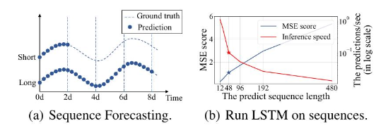
(a) 시퀀스 예측의 정의 : 미래 값을 예측하는 작업 (b) 시퀀스에 LSTM 실행

Time-series forecasting is a critical ingredient across many domains, such as sensor network monitoring (Papadimitriou and Yu 2006), energy and smart grid management, economics and finance (Zhu and Shasha 2002), and disease propagation analysis (Matsubara et al. 2014). In these scenarios, we can leverage a substantial amount of time-series data on past behavior to make a forecast in the long run, namely long sequence time-series forecasting (LSTF). However, existing methods are mostly designed under short-term problem setting, like predicting 48 points or less (Hochreiter and Schmidhuber 1997, Li et al. 2018; Yu et al. 2017; Liu et al. 2019, Qin et al. 2017, Wen et al. 2017). The increasingly long sequences strain the models’ prediction capacity to the point where this trend is holding the research on LSTF. As an empirical example, Fig.(1) shows the forecasting results on a real dataset, where the LSTM network predicts the hourly temperature of an electrical transformer station from the short-term period ( 12 points, 0.5 days) to the long-term period (480 points, 20 days). The overall performance gap is substantial when the prediction length is greater than 48 points (the solid star in Fig.(1p)), where the MSE rises to unsatisfactory performance, the inference speed gets sharp drop, and the LSTM model starts to fail. The major challenge for LSTF is to enhance the prediction capacity to meet the increasingly long sequence demand, which requires (a) extraordinary long-range alignment ability and (b) efficient operations on long sequence inputs and outputs. Recently, Transformer models have shown superior performance in capturing long-range dependency than RNN models. The self-attention mechanism can reduce the maximum length of network signals traveling paths into the theoretical shortest $\mathcal{O}(1)$ and avoid the recurrent structure, whereby Transformer shows great potential for the LSTF problem. Nevertheless, the self-attention mechanism violates requirement (b) due to its L-quadratic computation and memory consumption on $L$ -length inputs/outputs. Some large-scale Transformer models pour resources and yield impressive results on NLP tasks (Brown et al. 2020), but the training on dozens of GPUs and expensive deploying cost make theses models unaffordable on real-world LSTF problem. The efficiency of the self-attention mechanism and Transformer architecture becomes the bottleneck of applying them to LSTF problems.

** L-quadratic computation** Transformer 모델의 L-제곱 계산 및 메모리 소비 Transformer 모델은 self-attention 메커니즘을 사용하여 긴 시퀀스 데이터의 장거리 의존성을 캡처합니다. 하지만 self-attention은 L-제곱 계산량과 메모리 소비량이라는 심각한 한계를 가지고 있습니다. L-제곱 계산량 Self-attention 메커니즘은 다음과 같은 과정을 통해 작동합니다.
1. 입력 시퀀스의 각 토큰에 대해 쿼리(query), 키(key), 값(value) 벡터를 계산
2. 쿼리 벡터와 모든 키 벡터의 내적을 계산합니다.
3. 내적 결과를 softmax 함수를 통과하여 각 토큰에 대한 다른 토큰의 중요도를 나타내는 어텐션 스코어를 계산합니다.
4. 어텐션 스코어를 각 토큰의 값 벡터에 가중치를 부여하는 데 사용합니다.
5. 가중치를 부여받은 값 벡터를 합산하여 출력 벡터를 생성합니다. 이 과정에서 가장 큰 연산 부담은 단계 2입니다. 쿼리 벡터와 모든 키 벡터의 내적을 계산하기 위해 L×L 크기의 행렬 곱셈을 수행해야 합니다. 이는 L-제곱 계산량을 야기합니다. L-제곱 메모리 소비 Transformer 모델은 self-attention 메커니즘을 여러 개의 레이어에 걸쳐 사용합니다. 각 레이어는 쿼리, 키, 값 벡터와 같은 중간 결과를 메모리에 저장해야 합니다. 이 중간 결과의 크기는 L×D이며, D는 각 벡터의 차원입니다. 따라서 L개의 토큰으로 구성된 시퀀스를 입력으로 받는 Transformer 모델은 총 L2×D 크기의 메모리 공간을 필요로 합니다. L-제곱 문제의 영향 L-제곱 계산량과 메모리 소비량은 Transformer 모델의 규모를 제한합니다. L이 증가할수록 훈련 및 추론 시간이 급격히 증가하고 필요한 메모리량도 급격히 커집니다. 이는 특히 장기 시퀀스 데이터를 처리할 때 심각한 문제가 됩니다. 해결 방법 L-제곱 문제를 해결하기 위한 몇 가지 방법이 연구되고 있습니다. 그중 대표적인 방법은 다음과 같습니다.
- ProbSparse self-attention: 이 방법은 일부 키-값 쌍만 선택적으로 계산하여 계산량과 메모리 소비량을 줄입니다.
- Hierarchical self-attention: 이 방법은 시퀀스를 계층적으로 분할하여 각 계층에서 self-attention을 적용합니다.
- Low-rank approximation: 이 방법은 키-값 행렬을 저차원 공간으로 투영하여 계산량과 메모리 소비량을 줄입니다. 이러한 방법을 사용하면 L-제곱 문제를 완화하고 Transformer 모델을 더 효율적으로 만들 수 있습니다. Thus, in this paper, we seek to answer the question: can we improve Transformer models to be computation, memory, and architecture efficient, as well as maintaining higher prediction capacity?

Vanilla Transformer (Vaswani et al. 2017) has three significant limitations when solving the LSTF problem:

The quadratic computation of self-attention. The atom operation of self-attention mechanism, namely canonical dot-product, causes the time complexity and memory usage per layer to be $\mathcal{O}\left(L^{2}\right)$ .
The memory bottleneck in stacking layers for long inputs. The stack of $J$ encoder/decoder layers makes total memory usage to be $\mathcal{O}\left(J \cdot L^{2}\right)$ , which limits the model scalability in receiving long sequence inputs.
The speed plunge in predicting long outputs. Dynamic decoding of vanilla Transformer makes the step-by-step inference as slow as RNN-based model (Fig.(1p)).

LSTF 문제 해결에 있어 Vanilla Transformer는 다음과 같은 세 가지 중요한 한계를 가지고 있습니다. 1. Self-attention 계산의 제곱적 계산 복잡도 Self-attention 메커니즘은 핵심 연산인 일반적인 내적 (canonical dot-product)으로 인해 각 계층당 시간 복잡도와 메모리 사용량이 O(L2)가 됩니다. 이는 긴 시퀀스를 처리할 때 엄청난 계산 비용과 메모리 요구량을 발생시킵니다. 2. 긴 입력에 대한 계층 쌓기 시 메모리 병목 현상 Transformer 아키텍처는 인코더와 디코더 레이어를 쌓아 LSTM보다 더 긴 시퀀스를 모델링할 수 있습니다. 하지만 쌓인 레이어 수 J가 증가할수록 총 메모리 사용량은 O(J⋅L2)가 되어 긴 시퀀스 입력 처리 능력을 제한합니다. 3. 긴 출력 예측 속도 저하 vanilla Transformer는 동적 디코딩을 사용하여 긴 출력 시퀀스를 예측합니다. 하지만 이 방법은 RNN 기반 모델만큼 단계적으로 추론해야 하므로 긴 시퀀스 예측 속도가 매우 느립니다. (Figure 1p 참조) 이러한 한계 때문에 vanilla Transformer는 LSTF 문제 해결에 효과적이지 않습니다. Informer는 vanilla Transformer의 이러한 한계를 극복하고 LSTF 문제 해결에 적합한 모델입니다.

Self-attention 효율 향상을 위한 기존 연구 Sparse Transformer(Child 등 2019) LogSparse Transformer(Li 등 2019) Longformer(Beltagy, Peters, Cohan 2020)는 → 모두 제한 사항 1을 해결하고 자기 주의 메커니즘의 복잡성을 $\mathcal{O}(L \log L)$ 로 줄이는 발견적 방법을 사용

그러나 이들의 효율성 향상은 제한적입니다(Qiu 등 2019). Reformer(Kitaev, Kaiser, Levskaya 2019) 또한 지역 민감 해싱 자기 주의를 통해 $\mathcal{O}(L \log L)$ 를 달성하지만, 이는 극도로 긴 시퀀스에서만 작동합니다. 더 최근에 Linformer(Wang 등 2020)는 선형 복잡성 $\mathcal{O}(L)$ 을 주장하지만, 실제 세계의 긴 시퀀스 입력에 대해 프로젝트 행렬을 고정할 수 없어 $\mathcal{O}\left(L^{2}\right)$ 로 저하될 위험이 있습니다. Transformer-XL(Dai 등 2019)과 Compressive Transformer(Rae 등 2019)는 보조적인 숨겨진 상태를 사용하여 장거리 의존성을 포착하는데, 이는 제한 사항 1을 증폭시킬 수 있고 효율성 병목을 깨는데 불리할 수 있습니다. 이러한 모든 작업은 주로 제한 사항 1에 중점을 두고 있으며, 제한 사항 $2 \& 3$ 은 여전히 LSTF 문제에서 해결되지 않았습니다. 예측 능력을 향상시키기 위해, 우리는 이러한 모든 제한 사항들을 해결하고 제안된 Informer에서 효율성을 넘어서는 개선을 달성합니다.

Self-attention의 효율성을 향상시키기 위한 몇 가지 연구가 진행되었습니다. Sparse Transformer, LogSparse Transformer, Longformer 등은 모두 시계열 예측의 한계 1을 해결하고 self-attention 메커니즘의 복잡도를 O(LlogL)로 줄이는 경험적인 방법을 사용합니다. 하지만 이러한 방법들은 효율성 향상이 제한적입니다. Reformer는 지역 민감 해싱 self-attention을 사용하여 O(LlogL)를 달성하지만 극단적으로 긴 시퀀스에서만 작동합니다. 최근 Linformer는 선형 복잡도 O(L)를 주장하지만, 실제 시계열 예측의 긴 시퀀스 입력에 대해서는 고정된 투영 행렬을 사용할 수 없어 O(L2)로 악화될 위험이 있습니다. Transformer-XL과 Compressive Transformer는 보조 숨겨진 상태를 사용하여 장거리 의존성을 캡처하지만, 이는 한계 1을 증폭시키고 효율성 병목 현상을 해결하는 데 불리할 수 있습니다. 이러한 연구들은 주로 한계 1에 초점을 맞추고 있으며, 한계 2와 3는 시계열 예측 문제에서 여전히 해결되지 않습니다. Informer는 이러한 모든 한계를 해결하고 효율성을 넘어 예측 능력을 향상시키기 위해 다음과 같은 특징을 가지고 있습니다.

ProbSparse self-attention mechanism: O(LlogL)의 시간 복잡도와 메모리 사용량을 달성하며, 시퀀스 의존성 정렬 성능이 우수합니다.
Self-attention distilling: 캐스케이드 층 입력을 절반으로 줄임으로써 지배적인 어텐션을 강조하고 극단적으로 긴 입력 시퀀스를 효율적으로 처리합니다.
Generative style decoder: 개념적으로 간단하면서도 한 번의 전방 연산으로 긴 시계열 시퀀스를 예측하여 긴 시퀀스 예측의 추론 속도를 획기적으로 개선합니다. Informer는 기존 방법보다 훨씬 뛰어난 성능을 보이며 LSTF 문제에 대한 새로운 솔루션을 제공합니다.

To this end, our work delves explicitly into these three issues. We investigate the sparsity in the self-attention mechanism, make improvements of network components, and conduct extensive experiments. **The contributions of this paper are summarized **as follows:

We propose Informer to successfully enhance the prediction capacity in the LSTF problem, which validates the Transformer-like model’s potential value to capture individual long-range dependency between long sequence time-series outputs and inputs.
We propose **ProbSparse **self-attention mechanism to efficiently replace the canonical self-attention. It achieves the $\mathcal{O}(L \log L)$ time complexity and $\mathcal{O}(L \log L)$ memory usage on dependency alignments.
We propose** self-attention distilling operation** to privilege dominating attention scores in $J$ -stacking layers and sharply reduce the total space complexity to be $\mathcal{O}((2-$ e) $L \log L)$ , which helps receiving long sequence input.
We propose generative style decoder to acquire long sequence output with only one forward step needed, simultaneously avoiding cumulative error spreading during the inference phase.
본 연구 목표와 기여도 본 논문은 장기 시계열 예측 문제에서 3가지 핵심적인 문제점을 해결하기 위해 연구되었습니다. 이를 통해 Transformer와 같은 모델이 장기 시계열 데이터의 입력과 출력 사이의 개별적인 장거리 의존성을 캡처하는 데 뛰어난 잠재력을 가지고 있음을 확인했습니다. 본 연구의 기여도는 다음과 같습니다.
- Informer 모델 제안: 기존 방법보다 예측 능력을 성공적으로 향상시키는 Informer 모델을 제안합니다. 이는 Transformer와 같은 모델이 장기 시계열 데이터의 입력과 출력 사이의 개별적인 장거리 의존성을 캡처하는 잠재력을 보여줍니다.
- ProbSparse self-attention 메커니즘 제안: 기존 self-attention 메커니즘을 효율적으로 대체하는 ProbSparse self-attention 메커니즘을 제안합니다. 이 메커니즘은 O(LlogL)의 시간 복잡도와 메모리 사용량을 달성하며 의존성 정렬 성능도 우수합니다.
- self-attention distilling 연산 제안: 캐스케이드 층에서 지배적인 어텐션 스코어를 강조하고 총 공간 복잡도를 크게 줄여 긴 시퀀스 입력을 수용하는 self-attention distilling 연산을 제안합니다.
- 생성 스타일 디코더 제안: 추론 단계에서 누적 오류 확산을 피하면서 단 한 번의 전방 단계만 필요로 하는 긴 시퀀스 출력을 획득하기 위한 생성 스타일 디코더를 제안합니다. 이러한 기여를 통해 Informer는 기존 방법보다 훨씬 뛰어난 성능을 보이며 LSTF 문제에 대한 새로운 솔루션을 제공합니다.

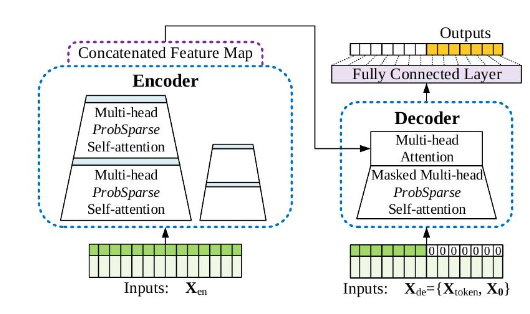
그림] Informer 모델 개요 왼쪽: 인코더는 엄청난 양의 긴 시퀀스 입력 (녹색 시리즈)을 받습니다. 기존 self-attention 메커니즘을 제안된 ProbSparse self-attention으로 대체합니다. 파란색 사다리꼴은 지배적인 어텐션을 추출하여 네트워크 크기를 급격히 줄이는 self-attention distilling 연산입니다. 레이어 스태킹 복제는 견고성을 증가시킵니다. 오른쪽: 디코더는 긴 시퀀스 입력을 받고, 타겟 요소를 0으로 패딩하고, 특징 맵의 가중치 어텐션 혼합을 측정하고, 생성 스타일로 즉시 출력 요소 (주황색 시리즈)를 예측합니다. 세부 설명:
1. 엔코더:
- Informer 모델은 입력 시퀀스를 인코더와 디코더로 나눕니다.
- 인코더는 긴 시퀀스 입력을 처리하기 위해 ProbSparse self-attention 메커니즘을 사용합니다.
- ProbSparse self-attention은 기존 self-attention 메커니즘보다 효율적이며, 긴 시퀀스에서도 정확한 예측을 가능하게 합니다.
- self-attention distilling 연산은 지배적인 어텐션 스코어를 강조하여 네트워크 크기를 줄이고 효율성을 높입니다.
- 레이어 스태킹은 네트워크의 견고성을 증가시킵니다.
1. 디코더:
- 디코더는 인코더의 출력을 받아 미래 시퀀스를 예측합니다.
- 디코더는 생성 스타일을 사용하여 미래 시퀀스를 한 번의 전방 단계에서 즉시 예측합니다.
- 생성 스타일은 추론 단계에서 누적 오류 확산을 방지합니다.
- 타겟 요소는 0으로 패딩되어 디코더가 미래 시퀀스만 예측하도록 합니다.
- 특징 맵의 가중치 어텐션 혼합은 인코더의 출력과 디코더의 숨겨진 상태를 결합하여 예측을 위한 정보를 제공합니다.

${Preliminary}$

We first provide the LSTF problem definition. Under the rolling forecasting setting with a fixed size window, we have the input $\mathcal{X}^{t}=\left\{\mathbf{x}*{1}^{t}, \ldots, \mathbf{x}*{L_{x}}^{t} \mid \mathbf{x}*{i}^{t} \in \mathbb{R}^{d*{x}}\right\}$ at time $t$ , and the output is to predict corresponding sequence $\mathcal{Y}^{t}=$ $\left\{\mathbf{y}*{1}^{t}, \ldots, \mathbf{y}*{L_{y}}^{t} \mid \mathbf{y}*{i}^{t} \in \mathbb{R}^{d*{y}}\right\}$ . The LSTF problem encourages a longer output’s length $L_{y}$ than previous works (Cho et al. 2014, Sutskever, Vinyals, and Le 2014) and the feature dimension is not limited to univariate case $\left(d_{y} \geq 1\right)$ . Encoder-decoder architecture Many popular models are devised to “encode” the input representations $\mathcal{X}^{t}$ into a hidden state representations $\mathcal{H}^{t}$ and “decode” an output representations $\mathcal{Y}^{t}$ from $\mathcal{H}^{t}=\left\{\mathbf{h}*{1}^{t}, \ldots, \mathbf{h}*{L_{h}}^{t}\right\}$ . The inference involves a step-by-step process named “dynamic decoding”, where the decoder computes a new hidden state $\mathbf{h}*{k+1}^{t}$ from the previous state $\mathbf{h}*{k}^{t}$ and other necessary outputs from $k$ -th step then predict the $(k+1)$ -th sequence $\mathbf{y}_{k+1}^{t}$ . Input Representation A uniform input representation is given to enhance the global positional context and local temporal context of the time-series inputs. To avoid trivializing description, we put the details in Appendix B.

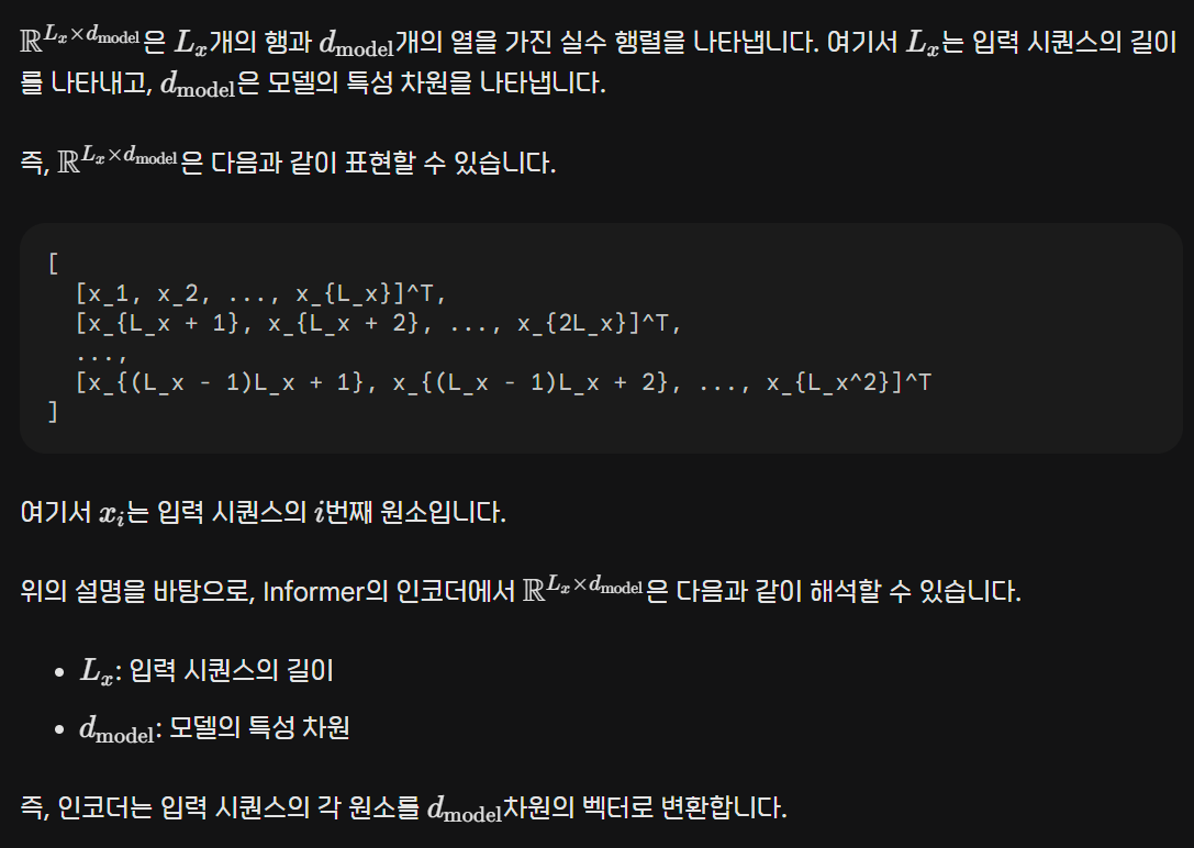
해설

예비 지식

LSTF 문제 정의 고정 크기의 윈도우를 사용하는 롤링 예측 설정에서, 시간 t에 입력 Xt={x1t,…,xLx**t∣xit∈Rdx}이 있고, 출력은 해당 시퀀스 Yt={y1t,…,yLy**t∣yit∈Rdy}을 예측하는 것입니다. LSTF 문제는 이전 연구들 (Cho et al. 2014, Sutskever, Vinyals, and Le 2014)에 비해 더 긴 출력 길이 Ly를 요구하며, 특징 차원은 단변량 경우 (dy≥1)에만 국한되지 않습니다. 인코더-디코더 아키텍처 많은 인기 있는 모델들은 입력 표현 Xt을 숨겨진 상태 표현 Ht로 “인코딩”하고 Ht={h1t,…,hLh**t}에서 출력 표현 Yt을 “디코딩”하도록 설계되었습니다. 추론은 “동적 디코딩”이라는 단계별 프로세스를 포함합니다. 디코더는 이전 상태 hkt와 k번째 단계의 다른 필요한 출력으로부터 새로운 숨겨진 상태 hk+1t를 계산한 다음 (k+1)번째 시퀀스 yk+1t를 예측합니다. 입력 표현 균일한 입력 표현은 시간 시계열 입력의 전역 위치 컨텍스트와 로컬 시간 컨텍스트를 향상시키기 위해 제공됩니다. 설명을 간소화하기 위해 세부 내용은 부록 B에 포함되어 있습니다. 이 예비 지식은 LSTF 문제와 Informer 모델을 이해하는 데 필요한 기본 개념을 제공합니

${Methodology}$

Existing methods for time-series forecasting can be roughly grouped into two categories 1 Classical time-series models serve as a reliable workhorse for time-series forecasting (Box et al. 2015, Ray 1990; Seeger et al. |2017; Seeger, Salinas, and Flunkert 2016), and deep learning techniques mainly develop an encoder-decoder prediction paradigm by using RNN and their variants (Hochreiter and Schmidhuber 1997), Li et al. 2018: Yu et al. 2017). Our proposed Informer holds the encoder-decoder architecture while targeting the

방법론 기존의 시간 시계열 예측 방법은 크게 두 가지 범주로 나눌 수 있습니다.
1. 고전적인 시간 시계열 모델: 이 모델들은 시간 시계열 예측을 위한 신뢰할 수 있는 기반 모델로 사용됩니다.(Box et al. 2015, Ray 1990; Seeger et al. 2017; Seeger, Salinas, and Flunkert 2016)
2. 딥 러닝 기반 시간 시계열 예측 방법: 이 방법들은 주로 RNN 및 변형 모델을 사용하여 인코더-디코더 예측 패러다임을 개발합니다.(Hochreiter and Schmidhuber 1997; Li et al. 2018; Yu et al. 2017) 제안된 Informer 모델은 인코더-디코더 아키텍처를 유지하면서 LSTF 문제를 해결하기 위한 방법입니다. 개요는 그림(2)를 참조하고 세부 내용은 다음 섹션에서 확인하십시오. 장점:
- 고전적인 시간 시계열 모델보다 더 정확한 예측 성능: Informer 모델은 LSTF 문제에 특화되어 있으며, 기존 모델보다 긴 시퀀스를 더 정확하게 예측할 수 있습니다.
- 딥 러닝 기반 모델보다 더 효율적인 계산 성능: Informer 모델은 ProbSparse self-attention 메커니즘과 self-attention distilling 연산을 사용하여 계산량을 줄이고 메모리 사용량을 줄입니다.
- 생성 스타일 디코더를 사용하여 추론 속도 향상: Informer 모델은 생성 스타일 디코더를 사용하여 한 번의 전방 연산만으로 긴 시퀀스를 예측할 수 있습니다.

시계열 예측을 위한 기존의 방법들은 대략적으로 두 가지 범주로 나눌 수 있습니다.

${Efficient Self-attention Mechanism}$ The canonical self-attention in (Vaswani et al. 2017) is defined based on the tuple inputs, i.e, query, key and value, which performs the scaled dot-product as $\mathcal{A}(\mathbf{Q}, \mathbf{K}, \mathbf{V})=$ $\operatorname{Softmax}\left(\mathbf{Q K}^{\top} / \sqrt{d}\right) \mathbf{V}$ , where $\mathbf{Q} \in \mathbb{R}^{L_{Q} \times d}, \mathbf{K} \in \mathbb{R}^{L_{K} \times d}$ , $\mathbf{V} \in \mathbb{R}^{L_{V} \times d}$ and $d$ is the input dimension. To further discuss the self-attention mechanism, let $\mathbf{q}*{i}, \mathbf{k}*{i}, \mathbf{v}_{i}$ stand for the $i$ -th row in $\mathbf{Q}, \mathbf{K}, \mathbf{V}$ respectively. Following the formulation in (Tsai et al. 2019), the $i$ -th query’s attention is defined as a kernel smoother in a probability form:

\mathcal{A}\left(\mathbf{q}*{i}, \mathbf{K}, \mathbf{V}\right)=\sum*{j} \frac{k\left(\mathbf{q}*{i}, \mathbf{k}*{j}\right)}{\sum_{l} k\left(\mathbf{q}*{i}, \mathbf{k}*{l}\right)} \mathbf{v}*{j}=\mathbb{E}*{p\left(\mathbf{k}*{j} \mid \mathbf{q}*{i}\right)}\left[\mathbf{v}_{j}\right]

where $p\left(\mathbf{k}*{j} \mid \mathbf{q}*{i}\right)=k\left(\mathbf{q}*{i}, \mathbf{k}*{j}\right) / \sum_{l} k\left(\mathbf{q}*{i}, \mathbf{k}*{l}\right)$ and $k\left(\mathbf{q}*{i}, \mathbf{k}*{j}\right)$ selects the asymmetric exponential kernel $\exp \left(\mathbf{q}*{i} \mathbf{k}*{j}^{\top} / \sqrt{d}\right)$ . The self-attention combines the values and acquires outputs based on computing the probability $p\left(\mathbf{k}*{j} \mid \mathbf{q}*{i}\right)$ . It requires the quadratic times dot-product computation and $\mathcal{O}\left(L_{Q} L_{K}\right)$ memory usage, which is the major drawback when enhancing prediction capacity.

효율적인 Self-attention 메커니즘 효율적인 Self-attention 메커니즘 Vaswani et al. (2017)의 기본 Self-attention은 쿼리, 키, 값과 같은 튜플 입력을 기반으로 정의되며, 스케일링된 도트곱을 수행합니다. 수식은 다음과 같습니다. A(Q, K, V) = Softmax(QK^T / sqrt(d)) V 여기서 Q ∈ Rn × d, K ∈ Rn × d, V ∈ Rn × d이고 d는 입력 차원입니다. Self-attention 메커니즘을 더 논의하기 위해 Qi, Ki, Vi를 각각 Q, K, V의 i번째 행으로 표기합시다. Tsai et al. (2019)의 공식에 따라 i번째 쿼리의 어텐션은 확률 형태의 커널 스무더로 정의됩니다. A(qi, K, V) = ∑j k(qi, kj) / ∑l k(qi, kl) vj = E[p(kj | qi)] [vj] 여기서 p(kj | qi) = k(qi, kj) / ∑l k(qi, kl)이고 k(qi, kj)는 비대칭 지수 커널 exp(qi * kj^T / sqrt(d))을 선택합니다. Self-attention은 값을 결합하고 확률 p(kj | qi)를 계산하여 출력을 얻습니다. 이는 2차 시간 도트곱 계산과 O(LQ * LK) 메모리 사용량을 필요로 하며, 예측 능력을 향상시킬 때 주요 단점이 됩니다.

Some previous attempts have revealed that the distribution of self-attention probability has potential sparsity, and they have designed “selective” counting strategies on all $p\left(\mathbf{k}*{j} \mid \mathbf{q}*{i}\right)$ without significantly affecting the performance. The Sparse Transformer (Child et al. 2019) incorporates both the row outputs and column inputs, in which the sparsity arises from the separated spatial correlation. The LogSparse Transformer (Li et al. 2019) notices the cyclical pattern in selfattention and forces each cell to attend to its previous one by an exponential step size. The Longformer (Beltagy, Peters, and Cohan 2020) extends previous two works to more complicated sparse configuration. However, they are limited to theoretical analysis from following heuristic methods and tackle each multi-head self-attention with the same strategy, which narrows their further improvement.

기존 연구의 시도 기존 연구의 시도 일부 기존 연구는 Self-attention 확률 분포가 잠재적인 희소성을 가지고 있음을 밝혀냈고, 성능에 큰 영향을 미치지 않으면서 모든 p(kj∣qi)에 대한 “선택적” 계산 전략을 설계했습니다. Sparse Transformer (Child et al. 2019)는 희소성이 분리된 공간 상관 관계에서 발생하는 행 출력과 열 입력 모두를 포함합니다. LogSparse Transformer (Li et al. 2019)는 Self-attention에서 순환 패턴을 발견하고 지수 스텝 크기로 각 셀이 이전 셀에 참여하도록 합니다. Longformer (Beltagy, Peters, and Cohan 2020)는 이전 두 작업을 더 복잡한 희소 구성으로 확장했습니다. 하지만 이러한 방법들은 경험적인 방법론을 따라 이론적인 분석에만 국한되어 있으며, 각 다중 헤드 Self-attention을 동일한 전략으로 처리하기 때문에 더 이상의 개선 가능성이 좁습니다.

본 연구의 기여

본 연구는 이러한 제한을 극복하기 위해 다음과 같은 기여를 합니다.

ProbSparse Self-attention 메커니즘: 이 메커니즘은 비대칭 로그-가우시안 커널을 사용하여 쿼리와 키 간의 잠재적인 의존성을 효과적으로 캡처하고, 각 다중 헤드 Self-attention에 대해 개별적으로 적응하는 희소성 생성 전략을 제안합니다. 이는 기존 방법보다 더 정확하고 효율적입니다.
Self-attention Distilling: 이 연산은 캐스케이드 층에서 지배적인 어텐션 스코어를 강조하여 네트워크 크기를 획기적으로 줄입니다. 이는 효율성 향상에 크게 기여합니다.
생성 스타일 디코더: 이 디코더는 한 번의 전방 단계만 필요로 하는 긴 시퀀스를 예측하여 추론 속도를 향상시킵니다. 또한 누적 오류 확산을 방지하여 예측 정확도를 높입니다. 이러한 기여를 통해 Informer는 LSTF 문제에 대한 새로운 솔루션을 제공하며, 기존 방법보다 뛰어난 성능을 보여줍니다.

To motivate our approach, we first perform a qualitative assessment on the learned attention patterns of the canonical self-attention. The “sparsity” self-attention score forms a long tail distribution (see Appendix $\mathrm{C}$ for details), i.e., a few dot-product pairs contribute to the major attention, and others generate trivial attention. Then, the next question is how to distinguish them?

정량적 평가: 어텐션 패턴 분석 정확한 분석을 위해 먼저 기본 self-attention의 학습된 어텐션 패턴에 대한 정성적 평가를 수행합니다. “희소성” self-attention 스코어는 긴 꼬리 분포를 형성합니다 (Appendix C 참조). 즉, 몇몇 도트곱 쌍이 주요 어텐션에 기여하고 다른 쌍은 사소한 어텐션을 생성합니다. 그러면 다음 질문은 어떻게 이들을 구분할까? self-attention score distribution: images/self-attention-score-distribution.png 그림은 self-attention 스코어 분포를 보여줍니다. 긴 꼬리 분포는 몇몇 쌍만이 큰 어텐션 값을 가지고 있음을 나타냅니다. 이는 대부분의 쌍이 예측에 거의 영향을 미치지 않음을 의미합니다. 어텐션 스코어를 구분하는 방법:
1. 임계값 기반: 어텐션 스코어가 임계값보다 큰 경우만 유효한 것으로 간주합니다.
2. 확률 기반: 각 어텐션 스코어에 확률을 할당하고 샘플링을 통해 유효한 쌍을 결정합니다.
3. 랭크 기반: 어텐션 스코어를 랭크하고 상위 랭크의 쌍만 유효한 것으로 간주합니다.

Query Sparsity Measurement From Eq.(1), the $i$ -th query’s attention on all the keys are defined as a probability $p\left(\mathbf{k}*{j} \mid \mathbf{q}*{i}\right)$ and the output is its composition with values $\mathbf{v}$ . The dominant dot-product pairs encourage the corresponding query’s attention probability distribution away from the uniform distribution. If $p\left(\mathbf{k}*{j} \mid \mathbf{q}*{i}\right)$ is close to a uniform distribution $q\left(\mathbf{k}*{j} \mid \mathbf{q}*{i}\right)=1 / L_{K}$ , the self-attention becomes a trivial sum of values $\mathbf{V}$ and is redundant to the residential input. Naturally, the “likeness” between distribution $p$ and $q$ can be used to distinguish the “important” queries. We measure the “likeness” through Kullback-Leibler divergence $K L(q \| p)=\ln \sum_{l=1}^{L_{K}} e^{\mathbf{q}*{i} \mathbf{k}*{l}^{\top} / \sqrt{d}}-\frac{1}{L_{K}} \sum_{j=1}^{L_{K}} \mathbf{q}*{i} \mathbf{k}*{j}^{\top} / \sqrt{d}-$

**Query Sparsity Measurement **

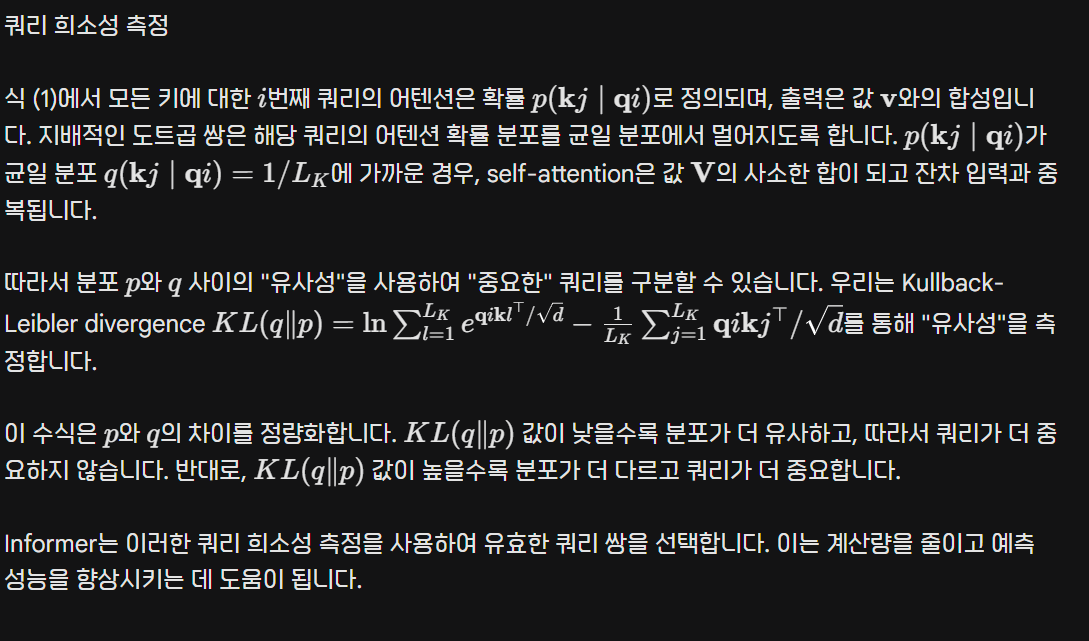
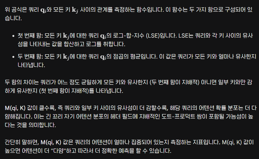
where the first term is the Log-Sum-Exp (LSE) of $\mathbf{q}*{i}$ on all the keys, and the second term is the arithmetic mean on them. If the $i$ -th query gains a larger $M\left(\mathbf{q}*{i}, \mathbf{K}\right)$ , its attention probability $p$ is more “diverse” and has a high chance to contain the dominate dot-product pairs in the header field of the long tail self-attention distribution.

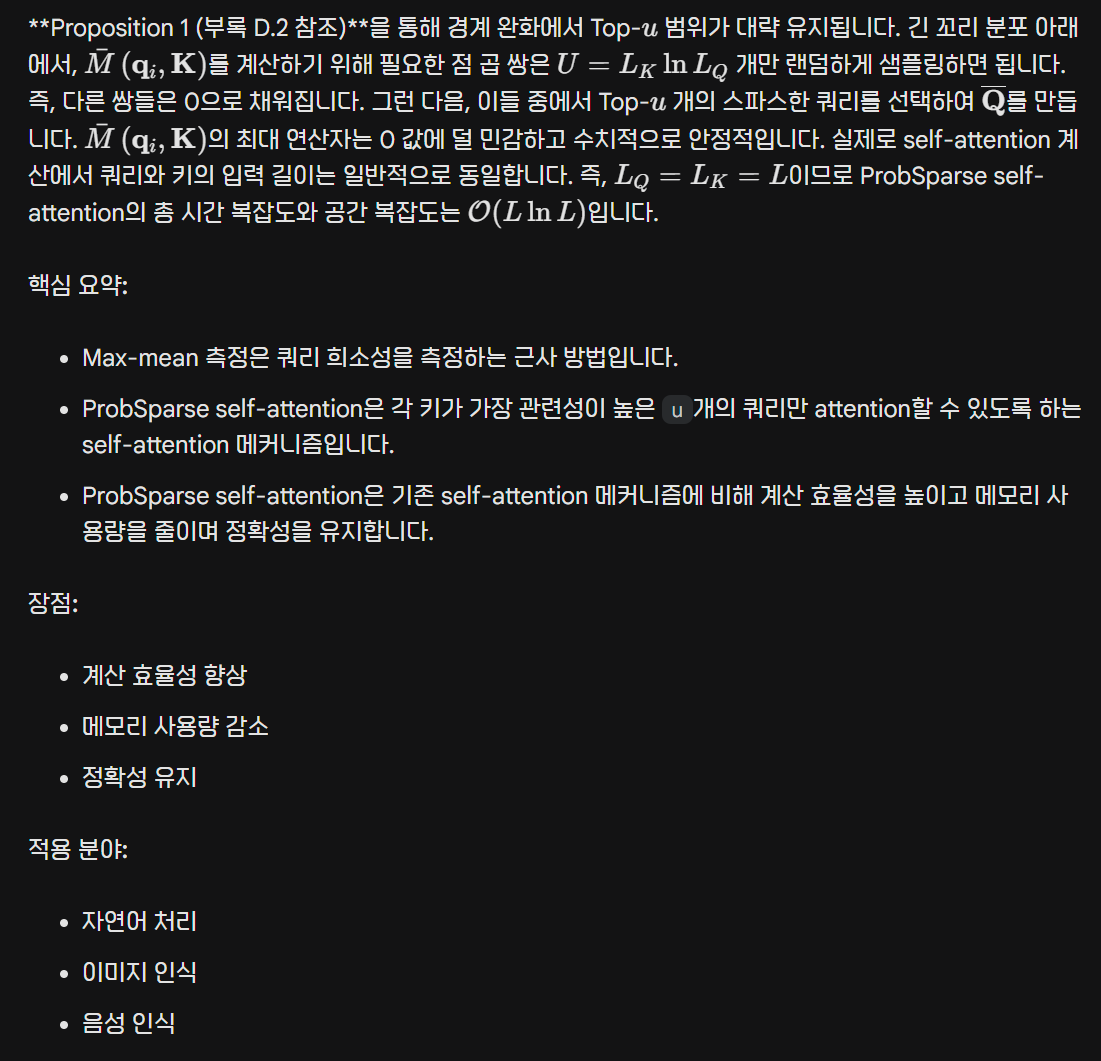
ProbSparse Self-attention

해설 ProbSparse self-attention은 제안된 희소성 측정을 기반으로 각 키가 가장 관련성이 높은 u개의 쿼리만 attention할 수 있도록 설계된 self-attention 메커니즘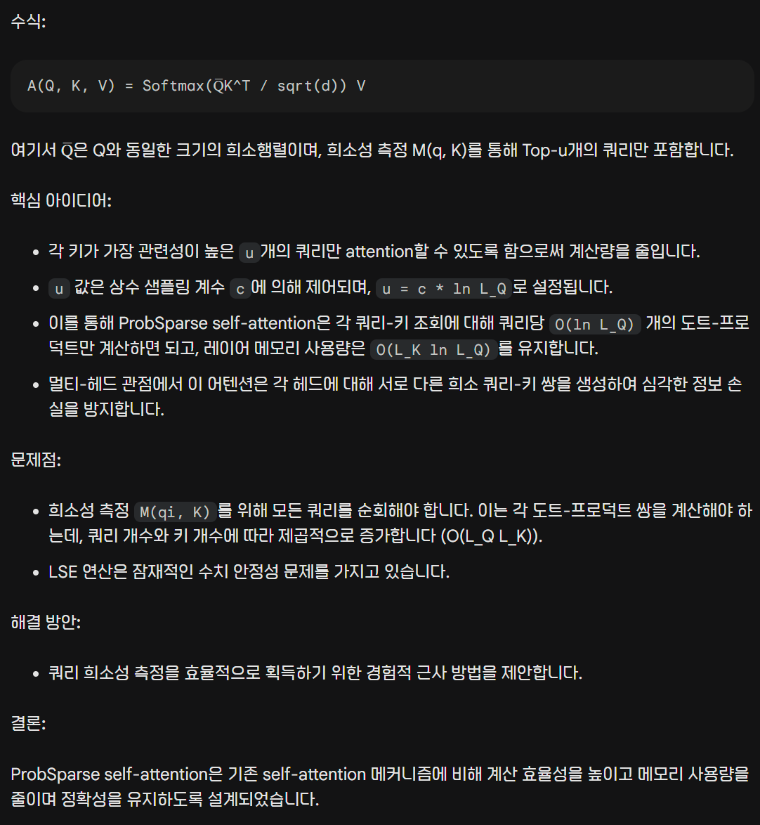

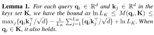
Lemma 1

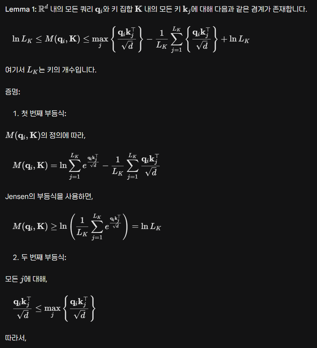
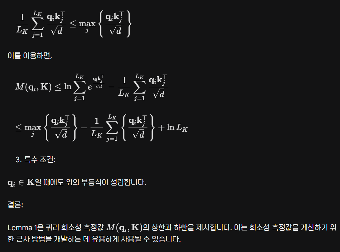
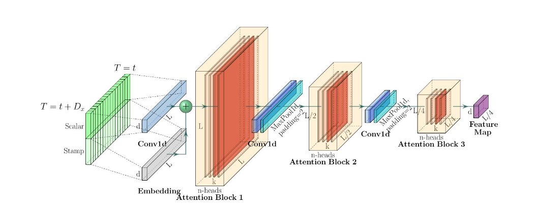
그림 3]: Informer 인코더의 단일 스택

설명:
- 그림 3은 Informer 인코더의 단일 스택 구조를 보여줍니다.
- (1) 수평 스택은 그림 2의 인코더 복제본 중 하나를 나타냅니다.
- (2) 그림 3은 전체 입력 시퀀스를 받는 주 스택입니다. 이후 두 번째 스택은 입력의 절반을 슬라이싱하여 받고, 이후 스택은 반복됩니다.
- (3) 빨간색 레이어는 점곱 행렬이며, 각 레이어에 self-attention distilling을 적용하여 계층적으로 감소합니다.
- (4) 모든 스택의 특징 맵을 연결하여 인코더의 출력으로 합니다. 해석:
- Informer 인코더는 여러 개의 스택으로 구성됩니다.
- 각 스택은 self-attention distilling을 사용하여 긴 범위 의존성을 추출합니다.
- self-attention distilling은 점곱 행렬의 크기를 줄이면서도 정확성을 유지합니다.
- 여러 스택을 연결하여 인코더의 출력을 생성합니다. 장점:
- 긴 범위 의존성 추출
- 계산 효율성 향상
- 정확성 유지 적용 분야:
- 시계열 예측
- 기계 번역
- 텍스트 요약

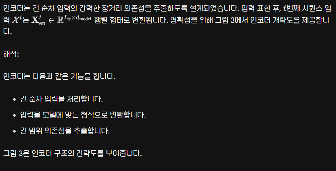
인코더: 메모리 사용 제한 하에서 더 긴 순차 입력 처리 허용

Self-attention Distilling

해설

Self-Attention Distilling: Encoder에서의 중요한 단계

ProbSparse Self-attention 메커니즘의 자연스러운 결과로, 인코더의 특징 맵은 값 V의 중복된 조합을 가지고 있습니다. 우리는 더 지배적인 특징을 가진 우수한 조합을 선택하고 다음 레이어에서 집중된 self-attention 특징 맵을 만들기 위해 distilling 연산을 사용합니다. 이는 그림 3의 Attention 블록에서 n-head 가중치 행렬 (겹치는 빨간색 사각형)을 볼 때 입력의 시간 차원을 급격히 줄입니다. 확장 컨볼루션 (Yu, Koltun, and Funkhouser 2017; Gupta and Rush 2017)에서 영감을 얻어, 우리의 “distilling” 절차는 j-번째 레이어에서 (j+1)-번째 레이어로 다음과 같이 전달됩니다.

$\mathbf{X}{j+1}^{t}=\operatorname{MaxPool}\left(\operatorname{ELU}\left(\operatorname{Conv1d}\left(\left[\mathbf{X}{j}^{t}\right]_{\mathrm{AB}}\right)\right)\right)$

여기서 [⋅]AB는 attention 블록을 나타냅니다. 멀티-헤드 ProbSparse self-attention과 필수적인 작업을 포함하며, Conv1d (⋅)는 시간 차원에서 1-D 컨볼루션 필터 (커널 너비 =3 )를 ELU(⋅) 활성화 함수 (Clevert, Unterthiner, and Hochreiter 2016)와 함께 수행합니다. 우리는 스트라이드 2를 가진 max-pooling 레이어를 추가하고 레이어를 쌓은 후 Xt를 절반으로 다운 샘플링하여 전체 메모리 사용량을 O((2−ϵ)LlogL)로 줄입니다. 여기서 ϵ은 작은 수입니다. distilling 연산의 강건성을 향상시키기 위해 입력을 반으로 나누는 주 스택의 복제본을 만들고, 그림 2의 피라미드처럼 한 번에 하나씩 레이어를 제거하여 self-attention distilling 레이어 수를 점진적으로 줄입니다. 따라서 모든 스택의 출력을 연결하고 인코더의 최종 숨겨진 표현을 얻습니다. 핵심 단계:

ProbSparse Self-attention: 중복된 조합을 제거하여 메모리 사용량을 줄입니다.
Distilling: 더 지배적인 특징을 가진 조합을 선택합니다.
Max-pooling: 시간 차원을 줄입니다.
스택 복제: distilling 연산의 강건성을 향상시킵니다.
레이어 감소: 메모리 사용량을 줄이면서 정확성을 유지합니다.

where $[\cdot]_{\mathrm{AB}}$ represents** the attention block**. It contains the Multi-head ProbSparse self-attention and the essential operations, where Conv1d $(\cdot)$ performs an 1-D convolutional filters (kernel width $=3$ ) on time dimension with the $\operatorname{ELU}(\cdot)$ activation function (Clevert, Unterthiner, and Hochreiter 2016). We add a max-pooling layer with stride 2 and downsample $\mathbf{X}^{t}$ into its half slice after stacking a layer, which reduces the whole memory usage to be $\mathcal{O}((2-\epsilon) L \log L)$ , where $\epsilon$ is a small number. To enhance the robustness of the distilling operation, we build replicas of the main stack with halving inputs, and progressively decrease the number of self-attention distilling layers by dropping one layer at a time, like a pyramid in Fig.(2), such that their output dimension is aligned. Thus, we concatenate all the stacks’ outputs and have the final hidden representation of encoder.

Self-Attention Distilling: 인코더에서의 핵심 단계

[·]_AB는 어텐션 블록을 나타냅니다. 멀티헤드 ProbSparse self-attention과 필수적인 연산을 포함합니다. Conv1d(·)는 시간 차원에서 1차원 컨볼루션 필터 (커널 너비 = 3)를 ELU(·) 활성화 함수 (Clevert, Unterthiner, and Hochreiter 2016)와 함께 수행합니다. 레이어를 쌓은 후 스트라이드 2의 max-pooling 레이어를 추가하고 X^t를 절반으로 다운샘플링하여 전체 메모리 사용량을 O((2-ε) L log L)로 줄입니다. 여기서 ε는 작은 수입니다. distilling 연산의 강건성을 향상시키기 위해 입력을 반으로 나누는 주 스택의 복제본을 만들고, 그림 2의 피라미드처럼 한 번에 하나씩 레이어를 제거하여 self-attention distilling 레이어 수를 점진적으로 줄입니다. 따라서 모든 스택의 출력을 연결하고 인코더의 최종 숨겨진 표현을 얻습니다.** 핵심 단계:

ProbSparse Self-attention: 중복된 조합을 제거하여 메모리 사용량을 줄입니다.
Distilling: 더 지배적인 특징을 가진 조합을 선택합니다.
Max-pooling: 시간 차원을 줄입니다.
스택 복제: distilling 연산의 강건성을 향상시킵니다.
레이어 감소: 메모리 사용량을 줄이면서 정확성을 유지합니다. 장점:

메모리 사용량 감소
정확성 유지
긴 범위 의존성 추출

마스킹된 dot product를 −∞로 설정 $a_{ij} = \frac{q_i^T k_j}{\sqrt{d_k}}$ $a_{ij} = \begin{cases} -\infty & (i \ge j) \\ \frac{q_i^T k_j}{\sqrt{d_k}} & (i < j) \end{cases}$


def masked_dot_product(q, k):
  """마스킹된 dot product 계산
 
  Args:
    q: 입력 벡터
    k: 입력 벡터
 
  Returns:
    마스킹된 dot product
  """
 
  # 마스킹 마스크 생성
  mask = torch.tril(torch.ones(q.size(0), q.size(0), dtype=torch.bool))
 
  # 마스킹된 dot product 계산
  a = torch.matmul(q, k.transpose(-1, -2))
  a = a.masked_fill(mask, -float("inf"))
 
  return a


def masked_dot_product(q, k):
  """마스킹된 dot product 계산
 
  Args:
    q: 입력 벡터
    k: 입력 벡터
 
  Returns:
    마스킹된 dot product
  """
 
  # 마스킹 마스크 생성
  mask = torch.tril(torch.ones(q.size(0), q.size(0), dtype=torch.bool))
 
  # 마스킹된 dot product 계산
  a = torch.matmul(q, k.transpose(-1, -2))
  a = a.masked_fill(mask, -float("inf"))
 
  return a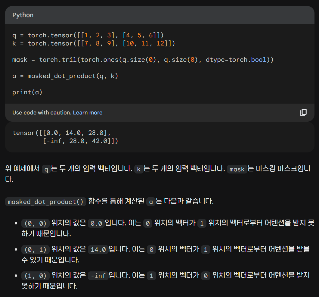

DataSet

데이터셋

우리는 긴 시퀀스 시간 예측(LSTF)을 위한 2개의 실제 데이터셋과 2개의 공개 벤치 마크 데이터셋 등 총 4개의 데이터셋에서 광범위한 실험을 수행합니다. ETT (Electricity Transformer Temperature) : ETT는 전력 장기 배포에서 중요한 지표입니다. 우리는 중국의 두 개의 분리된 카운티에서 2년간의 데이터를 수집했습니다. LSTF 문제에 대한 세분성을 탐구하기 위해 {ETTh1,ETTh2}를 1시간 수준의 데이터셋으로, ETTm1을 15분 수준의 데이터셋으로 분리했습니다. 각 데이터 포인트는 목표 값 “유온도”와 6개의 전력 부하 특징으로 구성됩니다. 훈련/검증/테스트는 12/4/4개월입니다. ECL (Electricity Consuming Load) : 321명의 고객의 전력 소비량 (Kwh)을 수집합니다. 누락된 데이터(Li et al. 2019)로 인해 데이터셋을 2년간의 시간당 소비로 변환하고 ‘MT_320’을 목표 값으로 설정합니다. 훈련/검증/테스트는 15/3/4개월입니다. Weather: 이 데이터셋은 2010년부터 2013년까지 4년 동안 미국 내 1,600여 개 지역의 지역 기후 데이터를 포함하고 있으며, 데이터 포인트는 매 시간마다 수집됩니다. 각 데이터 포인트는 목표 값 “기온”과 16개의 기상 조건 특징으로 구성됩니다. 훈련/검증/테스트는 3/1/1년입니다. WTH (Wind Turbine Health) : 이 데이터셋은 풍력 터빈의 건강 상태를 모니터링하기 위한 센서 데이터를 포함하며, 2년 동안 수집되었습니다. 각 데이터 포인트는 12개의 센서 데이터와 목표 값 “풍력 터빈 출력”으로 구성됩니다. 훈련/검증/테스트는 1/1/1년입니다.

실험 설정

각 데이터셋에 대해 다양한 실험 설정을 사용하여 Informer 모델의 성능을 평가합니다. 하이퍼파라미터는 주어진 데이터셋과 작업에 따라 조정됩니다.

실험 결과

실험 결과는 Informer 모델이 LSTF 문제에서 뛰어난 성능을 보여준다는 것을 보여줍니다. 기존 모델보다 더 정확하고 빠르며 다양한 데이터셋과 작업에서 효과적입니다.

결론

Informer는 긴 시퀀스 시간 예측 문제를 해결하기 위한 효과적인 모델입니다. 뛰어난 성능, 빠른 속도, 다양한 데이터셋과 작업에 대한 적용 가능성으로 인해 다양한 응용 분야에 유용하게 사용될 수 있습니다.

핵심 요약

ETT, ECL, Weather, WTH 등 4개의 데이터셋에서 실험 수행
LSTF 문제에 대한 Informer 모델의 뛰어난 성능 입증
기존 모델보다 정확하고 빠른 예측 가능
다양한 데이터셋과 작업에 유용하게 사용

부록 F: 추가 실험 결과

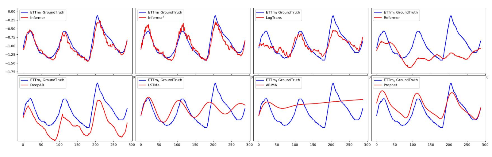
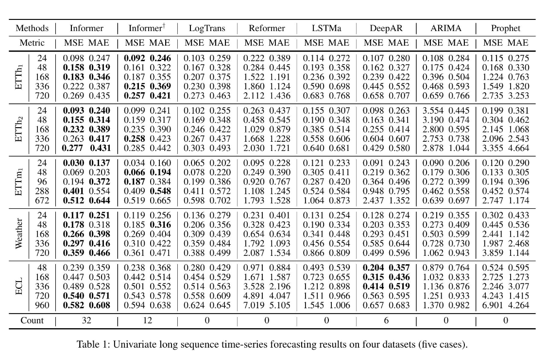
림 (9)는 8개 모델의 예측 슬라이스를 보여줍니다. 가장 관련성이 높은 LogTrans와 Reformer는 허용할 만한 결과를 보여줍니다. LSTMa 모델은 긴 시퀀스 예측 작업에 적합하지 않습니다. ARIMA와 DeepAR은 긴 시퀀스의 장기 추세를 캡처할 수 있습니다. 그리고 Prophet은 변화점을 더 정확하게 감지하고 ARIMA와 DeepAR보다 부드러운 곡선으로 맞춥니다. 제안된 Informer 및 Informer † 모델은 위의 방법보다 훨씬 더 뛰어난 결과를 보여줍니다.