Skip to Content

3주차 - Autoformer (NeurIPS 2021) (1)

https://jamboard.google.com/d/10z-N93YK9NZAWKo_ori9pLmd8a6boJiexYUhb4oHdvU/edit?usp=sharing 

Efficient computation

Auto-correlation을 계산하는 것은 O(L2)O\left(L^{2}\right) 의 복잡도를 가짐

Rxx(τ)=limL1Lt=1Lxtxtτ\mathcal{R}{x x}(\tau)=\lim {L \rightarrow \infty} \frac{1}{L} \sum{t=1}^{L} x{t} x_{t-\tau}

Time delay aggregation을 계산하는 것은 O(LlogL)O(L \log L) 의 복잡도를 가짐

τ1,,τk=argTopkτ{1,,L}(RQ,K(τ))R^Q,K(τ1),,R^Q,K(τk)=SoftMax(RQ,K(τ1),,RQ,K(τk)) Auto-Correlation (Q,K,V)=ikRoll(V,τi)R^Q,K(τi)\begin{gathered} \tau_{1}, \cdots, \tau_{k}=\underset{\tau \in\{1, \cdots, L\}}{\arg \operatorname{Topk}}\left(\mathcal{R}{Q, \mathcal{K}}(\tau)\right) \\ \hat{\mathcal{R}}{Q, \mathcal{K}}\left(\tau_{1}\right), \cdots, \widehat{\mathcal{R}}{Q, \mathcal{K}}\left(\tau{k}\right)=\operatorname{SoftMax}\left(\mathcal{R}{Q, \mathcal{K}}\left(\tau{1}\right), \cdots, \mathcal{R}{Q, \mathcal{K}}\left(\tau{k}\right)\right) \\ \text { Auto-Correlation }(Q, \mathcal{K}, \mathcal{V})=\sum_{i}^{k} \operatorname{Roll}\left(\mathcal{V}, \tau_{i}\right) \widehat{\mathcal{R}}{Q, \mathcal{K}}\left(\tau{i}\right) \end{gathered} 따라서 해당 Auto-Correlation Mechanism의 복잡도는 O(L2)\boldsymbol{O}\left(\boldsymbol{L}^{2}\right)

→ Fast Fourier Transform 으로 효율화


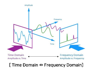
Fourier Transform

같은 형태를 반복하는 주기를 가진 파동은, 아무리 복잡한 것이라도 단순한 파동들이 결합 ( 복잡한 파동 )=( 단순한 파동 1)+( 단순한 파동 2)+( 단순한 파동 3)+ 임의의 주기함수 f(t)=a0+a1cos2πTt+a2cos2π2Tt+ancos2πnTt+b1sin2πTt+b2sin2π2Tt++bnsin2πnTt=a0+n=1(ancos2πnTt+bnsin2πnTt) \begin{aligned} & (\text { 복잡한 파동 })=(\text { 단순한 파동 } 1)+(\text { 단순한 파동 } 2)+(\text { 단순한 파동 } 3)+ \\ & \text { 임의의 주기함수 } f(t)=a_{0}+a_{1} \cos \frac{2 \pi}{T} t+a_{2} \cos \frac{2 \pi \cdot 2}{T} t+\cdots a_{n} \cos \frac{2 \pi \cdot n}{T} t \\ & +b_{1} \sin \frac{2 \pi}{T} t+b_{2} \sin \frac{2 \pi \cdot 2}{T} t+\cdots+b_{n} \sin \frac{2 \pi \cdot n}{T} t \\ & =a_{0}+\sum_{n=1}^{\infty}\left(a_{n} \cos \frac{2 \pi \cdot n}{T} t+\underline{b_{n}} \sin \frac{2 \pi \cdot n}{T} t\right) \\ & \ \end{aligned}
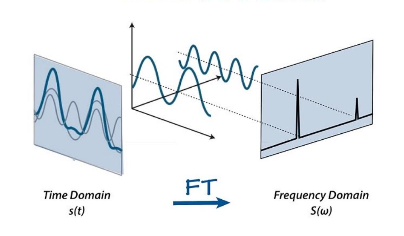

Fourier Transform vs Inverse Fourier Transform


Wiener-Khintchine Theorm

For a well behaved stationary random process the power spectrum is equal to the Fourier transform of the autocorrelation function.

Sx(ejω)=k=Rx(k)ejωkS_{x}\left(e^{j \omega}\right)=\sum_{k=-\infty}^{\infty} R_{x}(k) e^{-j \omega k}

Sx(ejω)=limN12N+1E[XN(ejω)2]=limN12N+1E[(n=NNx(n)ejωn)(k=NNx(k)ejωk)]=limN12N+1E[n=NNk=NNx(n)x(k)ejω(nk)]=limN12N+1n=NNk=NNE[x(n)x(k)]ejω(nk)=limN12N+1n=NNk=NNRx(nk)ejω(nk)=limNlimM12N+1n=NNk=MMRx(nk)ejω(nk)=limN12N+1n=NNlimMk=MMRx(nk)ejω(nk)=limN12N+1n=NN(k=Rx(k)ejωk)=(k=Rx(k)ejωk)limN12N+1n=NN1=k=Rx(k)ejωk\begin{aligned} S_{x}\left(e^{j \omega}\right) & =\lim {N \rightarrow \infty} \frac{1}{2 N+1} E\left[\left|X{N}\left(e^{j \omega}\right)\right|^{2}\right] \\ & =\lim {N \rightarrow \infty} \frac{1}{2 N+1} E\left[\left(\sum{n=-N}^{N} x(n) e^{-j \omega n}\right)\left(\sum_{k=-N}^{N} x(k) e^{-j \omega k}\right)^{*}\right] \\ & =\lim {N \rightarrow \infty} \frac{1}{2 N+1} E\left[\sum{n=-N}^{N} \sum_{k=-N}^{N} x(n) x(k) e^{-j \omega(n-k)}\right] \\ & =\lim {N \rightarrow \infty} \frac{1}{2 N+1} \sum{n=-N}^{N} \sum_{k=-N}^{N} E[x(n) x(k)] e^{-j \omega(n-k)} \\ & =\lim {N \rightarrow \infty} \frac{1}{2 N+1} \sum{n=-N}^{N} \sum_{k=-N}^{N} R_{x}(n-k) e^{-j \omega(n-k)} \\ & =\lim {N \rightarrow \infty} \lim {M \rightarrow \infty} \frac{1}{2 N+1} \sum{n=-N}^{N} \sum{k=-M}^{M} R_{x}(n-k) e^{-j \omega(n-k)} \\ & =\lim {N \rightarrow \infty} \frac{1}{2 N+1} \sum{n=-N}^{N} \lim {M \rightarrow \infty} \sum{k=-M}^{M} R_{x}(n-k) e^{-j \omega(n-k)} \\ & =\lim {N \rightarrow \infty} \frac{1}{2 N+1} \sum{n=-N}^{N}\left(\sum_{k=-\infty}^{\infty} R_{x}(k) e^{-j \omega k}\right) \\ & =\left(\sum_{k=-\infty}^{\infty} R_{x}(k) e^{-j \omega k}\right) \lim {N \rightarrow \infty} \frac{1}{2 N+1} \sum{n=-N}^{N} 1 \\ & =\sum_{k=-\infty}^{\infty} R_{x}(k) e^{-j \omega k} \end{aligned}